---
id: unsupervised-tutorial
title: Word representations
---
A popular idea in modern machine learning is to represent words by vectors. These vectors capture hidden information about a language, like word analogies or semantic. It is also used to improve performance of text classifiers.

In this tutorial, we show how to build these word vectors with the fastText tool. To download and install fastText, follow the first steps of [the tutorial on text classification](https://fasttext.cc/docs/en/supervised-tutorial.html).

## Getting the data

In order to compute word vectors, you need a large text corpus. Depending on the corpus, the word vectors will capture different information. In this tutorial, we focus on Wikipedia's articles but other sources could be considered, like  news or Webcrawl (more examples [here](http://statmt.org/)). To download a raw dump of Wikipedia, run the following command:

```bash
wget https://dumps.wikimedia.org/enwiki/latest/enwiki-latest-pages-articles.xml.bz2
```

Downloading  the Wikipedia corpus takes some time. Instead, lets restrict our study to the  first 1 billion bytes of English Wikipedia. They can be found on Matt Mahoney's [website](http://mattmahoney.net/):

```bash
$ mkdir data
$ wget -c http://mattmahoney.net/dc/enwik9.zip -P data
$ unzip data/enwik9.zip -d data
```

A raw Wikipedia dump contains a lot of HTML / XML data. We pre-process it with the wikifil.pl script bundled with fastText (this script was originally developed by Matt Mahoney, and can be found on his [website](http://mattmahoney.net/)).

```bash
$ perl wikifil.pl data/enwik9 > data/fil9
```

We can check the file by running the following command:

```bash
$ head -c 80 data/fil9
anarchism originated as a term of abuse first used against early working class
```

The text is nicely pre-processed and can be used to learn our word vectors.

## Training word vectors

<!--DOCUSAURUS_CODE_TABS-->
<!--Command line-->
Learning  word vectors on this data can now be achieved with a single command:

```bash
$ mkdir result
$ ./fasttext skipgram -input data/fil9 -output result/fil9
```

To decompose this command line: ./fastext calls the binary fastText executable (see how to install fastText [here](https://fasttext.cc/docs/en/support.html)) with the 'skipgram' model  (it can also be 'cbow'). We then specify the requires options '-input' for the location of the data and '-output' for the location where the word representations will be saved.

While fastText is running,  the progress and estimated time to completion is shown on your screen.  Once the program finishes, there should be two files in the result directory:

```bash
$ ls -l result
-rw-r-r-- 1 bojanowski 1876110778 978480850 Dec 20 11:01 fil9.bin
-rw-r-r-- 1 bojanowski 1876110778 190004182 Dec 20 11:01 fil9.vec
```

The `fil9.bin` file is a binary file that stores the whole fastText model and can be subsequently loaded. The `fil9.vec` file is a text file that contains the word vectors, one per line for each word in the vocabulary:

```bash
$ head -n 4 result/fil9.vec
218316 100
the -0.10363 -0.063669 0.032436 -0.040798 0.53749 0.00097867 0.10083 0.24829 ...
of -0.0083724 0.0059414 -0.046618 -0.072735 0.83007 0.038895 -0.13634 0.60063 ...
one 0.32731 0.044409 -0.46484 0.14716 0.7431 0.24684 -0.11301 0.51721 0.73262 ...
```

The first line is a header containing the number of words and the dimensionality of the vectors. The subsequent lines are the word vectors for all words in the vocabulary, sorted by decreasing frequency.
<!--Python-->
Learning  word vectors on this data can now be achieved with a single command:
```py
>>> import fasttext
>>> model = fasttext.train_unsupervised('data/fil9')
```
While fastText is running,  the progress and estimated time to completion is shown on your screen. Once the training finishes, `model` variable contains information on the trained model, and can be used for querying:

```py
>>> model.words
[u'the', u'of', u'one', u'zero', u'and', u'in', u'two', u'a', u'nine', u'to', u'is', ...
```
It returns all words in the vocabulary, sorted by decreasing frequency. We can get the word vector by:
```py
>>> model.get_word_vector("the")
array([-0.03087516,  0.09221972,  0.17660329,  0.17308897,  0.12863874,
        0.13912526, -0.09851588,  0.00739991,  0.37038437, -0.00845221,
        ...
       -0.21184735, -0.05048715, -0.34571868,  0.23765688,  0.23726143],
      dtype=float32)
```

We can save this model on disk as a binary file:
```py
>>> model.save_model("result/fil9.bin")
```
and reload it later instead of training again:
```py
$ python
>>> import fasttext
>>> model = fasttext.load_model("result/fil9.bin")
```

<!--END_DOCUSAURUS_CODE_TABS-->

## Advanced readers: skipgram versus cbow

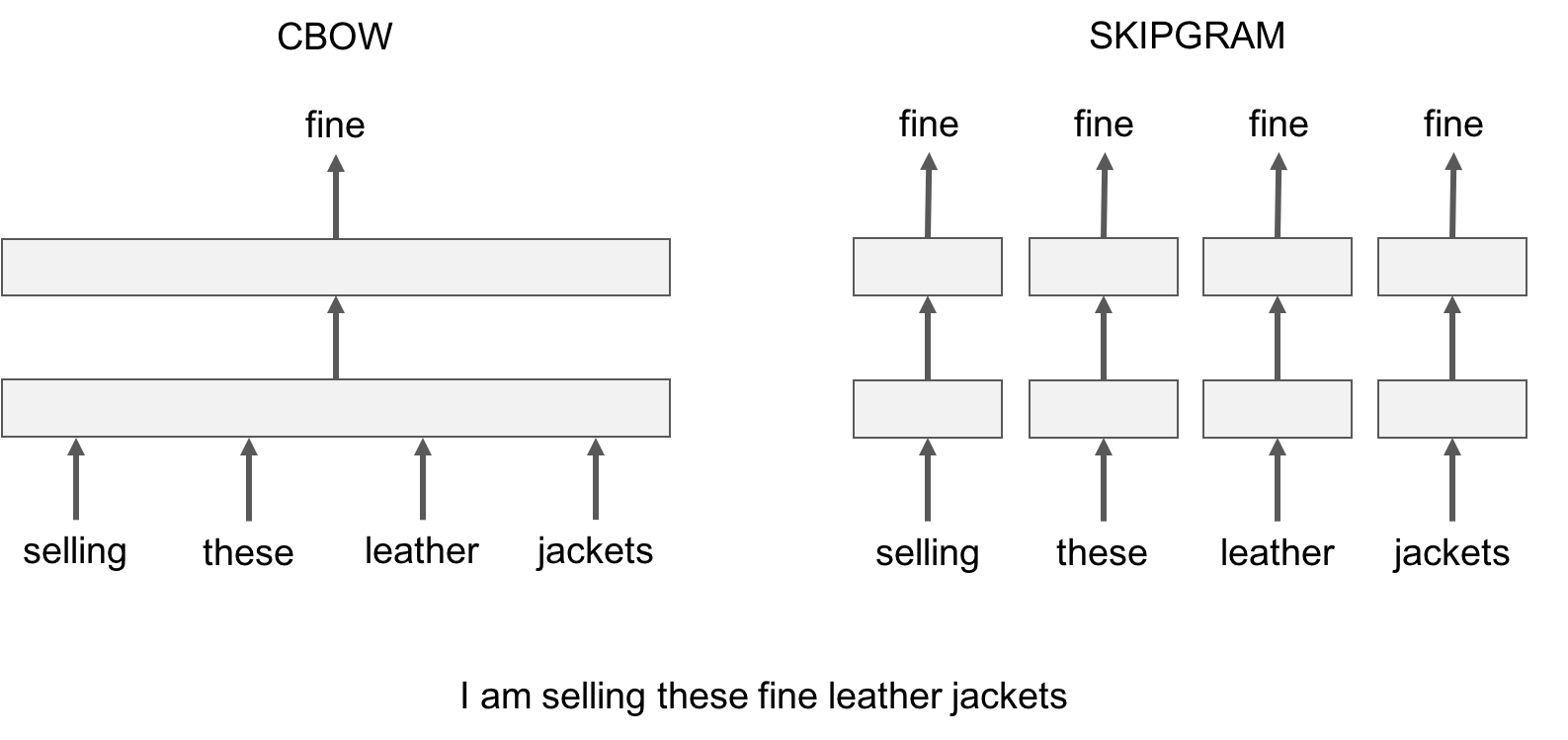
fastText provides two models for computing word representations: skipgram and cbow ('**c**ontinuous-**b**ag-**o**f-**w**ords').

The skipgram model learns to predict a target word thanks to a nearby word. On the other hand, the cbow model predicts the target word according to its context. The  context is represented as a bag of the  words contained in a fixed size window around the target word.

Let us illustrate this difference with an example:  given the sentence *'Poets have been mysteriously silent on the subject of cheese'* and the target word '*silent*', a skipgram model tries to predict the target using a random close-by word, like '*subject' *or* '*mysteriously*'**. *The cbow model takes all the words in a surrounding window, like {*been, *mysteriously*, on, the*}, and uses the sum of their vectors to predict the target. The figure below summarizes this difference with another example.

![cbow vs skipgram](https://fasttext.cc/img/cbo_vs_skipgram.png)
To train a cbow model with fastText, you run the following command:

<!--DOCUSAURUS_CODE_TABS-->
<!--Command line-->
```bash
./fasttext cbow -input data/fil9 -output result/fil9
```
<!--Python-->
```py
>>> import fasttext
>>> model = fasttext.train_unsupervised('data/fil9', "cbow")
```
<!--END_DOCUSAURUS_CODE_TABS-->

In practice, we observe that skipgram models works better with subword information than cbow.

## Advanced readers: playing with the parameters

So far, we run fastText with the default parameters, but depending on the data, these parameters may not be optimal. Let us give an introduction to some of the key parameters for word vectors.

The most important parameters of the model are its dimension and the range of size for the subwords. The dimension (*dim*) controls the size of the vectors, the larger they are the more information they can capture but requires more data to be learned. But, if they are too large, they are harder and slower to train. By default, we use 100 dimensions, but any value in the 100-300 range is as popular. The subwords are all the substrings contained in a word between the minimum size (*minn*) and the maximal size (*maxn*). By default, we take all the subword between 3 and 6 characters, but other range could be more appropriate to different languages:

<!--DOCUSAURUS_CODE_TABS-->
<!--Command line-->
```bash
$ ./fasttext skipgram -input data/fil9 -output result/fil9 -minn 2 -maxn 5 -dim 300
```
<!--Python-->
```py
>>> import fasttext
>>> model = fasttext.train_unsupervised('data/fil9', minn=2, maxn=5, dim=300)
```
<!--END_DOCUSAURUS_CODE_TABS-->

Depending on the quantity of data you have, you may want to change the parameters of the training.  The *epoch* parameter controls how many times the model will loop over your data. By default, we loop over the dataset 5 times.  If you dataset is extremely massive, you may want to loop over it less often. Another important parameter is the learning rate -*lr*. The higher the learning rate is, the faster the model converge to a solution but at the risk of overfitting to the dataset. The default value is 0.05 which is a good compromise. If you want to play with it we suggest to stay in the range of [0.01, 1]:

<!--DOCUSAURUS_CODE_TABS-->
<!--Command line-->
```bash
$ ./fasttext skipgram -input data/fil9 -output result/fil9 -epoch 1 -lr 0.5
```
<!--Python-->
```py
>>> import fasttext
>>> model = fasttext.train_unsupervised('data/fil9', epoch=1, lr=0.5)
```
<!--END_DOCUSAURUS_CODE_TABS-->

Finally , fastText is multi-threaded and uses 12 threads by default. If you have less CPU cores (say 4), you can easily set the number of threads using the *thread* flag:

<!--DOCUSAURUS_CODE_TABS-->
<!--Command line-->
```bash
$ ./fasttext skipgram -input data/fil9 -output result/fil9 -thread 4
```
<!--Python-->
```py
>>> import fasttext
>>> model = fasttext.train_unsupervised('data/fil9', thread=4)
```
<!--END_DOCUSAURUS_CODE_TABS-->


## Printing word vectors

Searching and printing word vectors directly from  the `fil9.vec`  file  is cumbersome. Fortunately, there is a `print-word-vectors` functionality in fastText.

For example, we can print the word vectors of words *asparagus,* *pidgey* and *yellow* with the following command:
<!--DOCUSAURUS_CODE_TABS-->
<!--Command line-->
```bash
$ echo "asparagus pidgey yellow" | ./fasttext print-word-vectors result/fil9.bin
asparagus 0.46826 -0.20187 -0.29122 -0.17918 0.31289 -0.31679 0.17828 -0.04418 ...
pidgey -0.16065 -0.45867 0.10565 0.036952 -0.11482 0.030053 0.12115 0.39725 ...
yellow -0.39965 -0.41068 0.067086 -0.034611 0.15246 -0.12208 -0.040719 -0.30155 ...
```
<!--Python-->
```py
>>> [model.get_word_vector(x) for x in ["asparagus", "pidgey", "yellow"]]
[array([-0.25751096, -0.18716481,  0.06921121,  0.06455903,  0.29168844,
        0.15426874, -0.33448914, -0.427215  ,  0.7813013 , -0.10600132,
        ...
        0.37090245,  0.39266172, -0.4555302 ,  0.27452755,  0.00467369],
      dtype=float32),
 array([-0.20613593, -0.25325796, -0.2422259 , -0.21067499,  0.32879013,
        0.7269511 ,  0.3782259 ,  0.11274897,  0.246764  , -0.6423613 ,
        ...
        0.46302193,  0.2530962 , -0.35795924,  0.5755718 ,  0.09843876],
      dtype=float32),
 array([-0.304823  ,  0.2543754 , -0.2198013 , -0.25421786,  0.11219151,
        0.38286993, -0.22636674, -0.54023844,  0.41095474, -0.3505803 ,
        ...
        0.54788435,  0.36740595, -0.5678512 ,  0.07523401, -0.08701935],
      dtype=float32)]

```
<!--END_DOCUSAURUS_CODE_TABS-->

A nice feature is that you can also query for words that did not appear in your data! Indeed words are represented by the sum of its substrings. As long as the unknown word is made of known substrings, there is a representation of it!

As an example let's try with a misspelled word:

<!--DOCUSAURUS_CODE_TABS-->
<!--Command line-->
```bash
$ echo "enviroment" | ./fasttext print-word-vectors result/fil9.bin
```
<!--Python-->
```py
>>> model.get_word_vector("enviroment")
```
<!--END_DOCUSAURUS_CODE_TABS-->

You still get a word vector for it! But how good it is? Let's find out in the next sections!


## Nearest neighbor queries

A simple way to check the quality of a word vector is to look at its nearest neighbors. This give an intuition of the type of semantic information the vectors are able to capture.

This can be achieved with the nearest neighbor (*nn*) functionality. For example, we can query the 10 nearest neighbors of a word by running the following command:

<!--DOCUSAURUS_CODE_TABS-->
<!--Command line-->
```bash
$ ./fasttext nn result/fil9.bin
Pre-computing word vectors... done.
```

Then we are prompted to type our query word, let us try *asparagus* :

```bash
Query word? asparagus
beetroot 0.812384
tomato 0.806688
horseradish 0.805928
spinach 0.801483
licorice 0.791697
lingonberries 0.781507
asparagales 0.780756
lingonberry 0.778534
celery 0.774529
beets 0.773984
```
<!--Python-->
```py
>>> model.get_nearest_neighbors('asparagus')
[(0.812384, u'beetroot'), (0.806688, u'tomato'), (0.805928, u'horseradish'), (0.801483, u'spinach'), (0.791697, u'licorice'), (0.781507, u'lingonberries'), (0.780756, u'asparagales'), (0.778534, u'lingonberry'), (0.774529, u'celery'), (0.773984, u'beets')]
```
<!--END_DOCUSAURUS_CODE_TABS-->

Nice! It seems that vegetable vectors are similar. Note that the nearest neighbor is the word *asparagus* itself, this means that this word appeared in the dataset. What about pokemons?

<!--DOCUSAURUS_CODE_TABS-->
<!--Command line-->
```bash
Query word? pidgey
pidgeot 0.891801
pidgeotto 0.885109
pidge 0.884739
pidgeon 0.787351
pok 0.781068
pikachu 0.758688
charizard 0.749403
squirtle 0.742582
beedrill 0.741579
charmeleon 0.733625
```
<!--Python-->
```py
>>> model.get_nearest_neighbors('pidgey')
[(0.891801, u'pidgeot'), (0.885109, u'pidgeotto'), (0.884739, u'pidge'), (0.787351, u'pidgeon'), (0.781068, u'pok'), (0.758688, u'pikachu'), (0.749403, u'charizard'), (0.742582, u'squirtle'), (0.741579, u'beedrill'), (0.733625, u'charmeleon')]
```
<!--END_DOCUSAURUS_CODE_TABS-->


Different evolution of the same Pokemon have close-by vectors! But what about our misspelled word, is its vector close to anything reasonable? Let s find out:

<!--DOCUSAURUS_CODE_TABS-->
<!--Command line-->
```bash
Query word? enviroment
enviromental 0.907951
environ 0.87146
enviro 0.855381
environs 0.803349
environnement 0.772682
enviromission 0.761168
realclimate 0.716746
environment 0.702706
acclimatation 0.697196
ecotourism 0.697081
```
<!--Python-->
```py
>>> model.get_nearest_neighbors('enviroment')
[(0.907951, u'enviromental'), (0.87146, u'environ'), (0.855381, u'enviro'), (0.803349, u'environs'), (0.772682, u'environnement'), (0.761168, u'enviromission'), (0.716746, u'realclimate'), (0.702706, u'environment'), (0.697196, u'acclimatation'), (0.697081, u'ecotourism')]
```
<!--END_DOCUSAURUS_CODE_TABS-->


Thanks to the information contained within the word, the vector of our misspelled word matches to reasonable words! It is not perfect but the main information has been captured.

## Advanced reader: measure of similarity

In order to find nearest neighbors, we need to compute a similarity score between words. Our words are represented by continuous word vectors and we can thus apply simple similarities to them. In particular we use the cosine of the angles between two vectors. This similarity is computed for all words in the vocabulary, and the 10 most similar words are shown.  Of course, if the word appears in the vocabulary, it will appear on top, with a similarity of 1.

## Word analogies

In a similar spirit, one can play around with word analogies. For example, we can see if our model can guess what is to France, and what Berlin is to Germany.





This can be done with the *analogies* functionality. It takes a word triplet (like *Germany Berlin France*) and outputs  the analogy:

<!--DOCUSAURUS_CODE_TABS-->
<!--Command line-->
```bash
$ ./fasttext analogies result/fil9.bin
Pre-computing word vectors... done.
Query triplet (A - B + C)? berlin germany france
paris 0.896462
bourges 0.768954
louveciennes 0.765569
toulouse 0.761916
valenciennes 0.760251
montpellier 0.752747
strasbourg 0.744487
meudon 0.74143
bordeaux 0.740635
pigneaux 0.736122
```
<!--Python-->
```py
>>> model.get_analogies("berlin", "germany", "france")
[(0.896462, u'paris'), (0.768954, u'bourges'), (0.765569, u'louveciennes'), (0.761916, u'toulouse'), (0.760251, u'valenciennes'), (0.752747, u'montpellier'), (0.744487, u'strasbourg'), (0.74143, u'meudon'), (0.740635, u'bordeaux'), (0.736122, u'pigneaux')]
```
<!--END_DOCUSAURUS_CODE_TABS-->

The answer provided by our model is *Paris*, which is correct. Let's have a look at a less obvious example:

<!--DOCUSAURUS_CODE_TABS-->
<!--Command line-->
```bash
Query triplet (A - B + C)? psx sony nintendo
gamecube 0.803352
nintendogs 0.792646
playstation 0.77344
sega 0.772165
gameboy 0.767959
arcade 0.754774
playstationjapan 0.753473
gba 0.752909
dreamcast 0.74907
famicom 0.745298
```
<!--Python-->
```py
>>> model.get_analogies("psx", "sony", "nintendo")
[(0.803352, u'gamecube'), (0.792646, u'nintendogs'), (0.77344, u'playstation'), (0.772165, u'sega'), (0.767959, u'gameboy'), (0.754774, u'arcade'), (0.753473, u'playstationjapan'), (0.752909, u'gba'), (0.74907, u'dreamcast'), (0.745298, u'famicom')]
```
<!--END_DOCUSAURUS_CODE_TABS-->


Our model considers that the *nintendo* analogy of a *psx* is the *gamecube*, which seems  reasonable. Of course the quality of the analogies depend on the dataset used to train the model and one can only hope to cover fields only in the dataset.


## Importance of character n-grams

Using subword-level information is particularly interesting to build vectors for unknown words. For example, the word *gearshift* does not exist on Wikipedia but we can still query its closest existing words:

<!--DOCUSAURUS_CODE_TABS-->
<!--Command line-->
```bash
Query word? gearshift
gearing 0.790762
flywheels 0.779804
flywheel 0.777859
gears 0.776133
driveshafts 0.756345
driveshaft 0.755679
daisywheel 0.749998
wheelsets 0.748578
epicycles 0.744268
gearboxes 0.73986
```
<!--Python-->
```py
>>> model.get_nearest_neighbors('gearshift')
[(0.790762, u'gearing'), (0.779804, u'flywheels'), (0.777859, u'flywheel'), (0.776133, u'gears'), (0.756345, u'driveshafts'), (0.755679, u'driveshaft'), (0.749998, u'daisywheel'), (0.748578, u'wheelsets'), (0.744268, u'epicycles'), (0.73986, u'gearboxes')]
```
<!--END_DOCUSAURUS_CODE_TABS-->



Most of the retrieved words share substantial substrings but a few are actually quite different, like *cogwheel*. You can try other words like *sunbathe* or *grandnieces*.

Now that we have seen the interest of subword information for unknown words, let's check how it compares to a model that does not use subword information. To train a model without subwords, just run the following command:

<!--DOCUSAURUS_CODE_TABS-->
<!--Command line-->
```bash
$ ./fasttext skipgram -input data/fil9 -output result/fil9-none -maxn 0
```
The results are saved in result/fil9-non.vec and result/fil9-non.bin.
<!--Python-->
```py
>>> model_without_subwords = fasttext.train_unsupervised('data/fil9', maxn=0)
```
<!--END_DOCUSAURUS_CODE_TABS-->


To illustrate the difference, let us take an uncommon word in Wikipedia, like *accomodation* which is a misspelling of *accommodation**.* Here is the nearest neighbors obtained without subwords:

<!--DOCUSAURUS_CODE_TABS-->
<!--Command line-->
```bash
$ ./fasttext nn result/fil9-none.bin
Query word? accomodation
sunnhordland 0.775057
accomodations 0.769206
administrational 0.753011
laponian 0.752274
ammenities 0.750805
dachas 0.75026
vuosaari 0.74172
hostelling 0.739995
greenbelts 0.733975
asserbo 0.732465
```
<!--Python-->
```py
>>> model_without_subwords.get_nearest_neighbors('accomodation')
[(0.775057, u'sunnhordland'), (0.769206, u'accomodations'), (0.753011, u'administrational'), (0.752274, u'laponian'), (0.750805, u'ammenities'), (0.75026, u'dachas'), (0.74172, u'vuosaari'), (0.739995, u'hostelling'), (0.733975, u'greenbelts'), (0.732465, u'asserbo')]
```
<!--END_DOCUSAURUS_CODE_TABS-->

The result does not make much sense, most of these words are unrelated. On the other hand, using subword information gives the following list of nearest neighbors:

<!--DOCUSAURUS_CODE_TABS-->
<!--Command line-->
```bash
Query word? accomodation
accomodations 0.96342
accommodation 0.942124
accommodations 0.915427
accommodative 0.847751
accommodating 0.794353
accomodated 0.740381
amenities 0.729746
catering 0.725975
accomodate 0.703177
hospitality 0.701426
```
<!--Python-->
```py
>>> model.get_nearest_neighbors('accomodation')
[(0.96342, u'accomodations'), (0.942124, u'accommodation'), (0.915427, u'accommodations'), (0.847751, u'accommodative'), (0.794353, u'accommodating'), (0.740381, u'accomodated'), (0.729746, u'amenities'), (0.725975, u'catering'), (0.703177, u'accomodate'), (0.701426, u'hospitality')]
```
<!--END_DOCUSAURUS_CODE_TABS-->

The nearest neighbors capture different variation around the word *accommodation*. We also get semantically related words such as *amenities* or *catering*.

## Conclusion

In this tutorial, we show how to obtain word vectors from Wikipedia. This can be done for any language and we provide [pre-trained models](https://fasttext.cc/docs/en/pretrained-vectors.html) with the default setting for 294 of them.