1
2
3
4
5
6
7
8
9
10
11
12
13
14
15
16
17
18
19
20
21
22
23
24
25
26
27
28
29
30
31
32
33
34
35
36
37
38
39
40
41
42
43
44
45
46
47
48
49
50
51
52
53
54
55
56
57
58
59
60
61
62
63
64
65
66
67
68
69
70
71
72
73
74
75
76
77
78
79
80
81
82
83
84
85
86
87
88
89
90
91
92
93
94
95
96
97
98
99
100
101
102
103
104
105
106
107
108
109
110
111
112
113
114
115
116
117
118
119
120
121
122
|
---
# Gyrotropic Media
---
In this example, we will perform simulations with gyrotropic media. See [Materials](../Materials.md#gyrotropic-media) for more information on how gyrotropy is supported.
[TOC]
### Faraday Rotation
Consider a uniform gyroelectric medium with bias vector $\mathbf{b} = b \hat{z}$. In the frequency domain, the *x* and *y* components of the dielectric tensor have the form
$$\epsilon = \begin{bmatrix}\epsilon_\perp & -i\eta \\ i\eta & \epsilon_\perp \end{bmatrix}$$
The skew-symmetric off-diagonal components give rise to [Faraday rotation](https://en.wikipedia.org/wiki/Faraday_effect): when a plane wave linearly polarized along *x* is launched along the gyrotropy axis *z*, the polarization vector will precess around the gyrotropy axis as the wave propagates. This is the principle behind [Faraday rotators](https://en.wikipedia.org/wiki/Faraday_rotator), devices that act as one-way valves for light.
A plane wave undergoing Faraday rotation can be described by the complex ansatz
$$\begin{bmatrix}E_x \\ E_y\end{bmatrix} = E_0 \begin{bmatrix}\cos(\kappa_c z) \\ \sin(\kappa_c z)\end{bmatrix} e^{i(kz-\omega t)}$$
where $\kappa_c$ is the Faraday rotation (in radians) per unit of propagation distance. Substituting this into the frequency domain Maxwell's equations, with the above dielectric tensor, yields
$$|\kappa_c| = \omega \sqrt{\frac{\mu}{2} \, \left(\epsilon_\perp - \sqrt{\epsilon_\perp^2 - \eta^2}\right)}$$
We model this phenomenon in the simulation script [faraday-rotation.py](https://github.com/NanoComp/meep/blob/master/python/examples/faraday-rotation.py). First, we define a gyroelectric material:
```python
import meep as mp
## Parameters for a gyrotropic Lorentzian medium
epsn = 1.5 # background permittivity
f0 = 1.0 # natural frequency
gamma = 1e-6 # damping rate
sn = 0.1 # sigma parameter
b0 = 0.15 # magnitude of bias vector
susc = [mp.GyrotropicLorentzianSusceptibility(frequency=f0, gamma=gamma, sigma=sn,
bias=mp.Vector3(0, 0, b0))]
mat = mp.Medium(epsilon=epsn, mu=1, E_susceptibilities=susc)
```
The `GyrotropicLorentzianSusceptibility` object has a `bias` argument that takes a `Vector3` specifying the gyrotropy vector. In this case, the vector points along *z*, and its magnitude (which specifies the precession frequency) is determined by the variable `b0`. The other arguments play the same role as in an ordinary (non-gyrotropic) [Lorentzian susceptibility](Material_Dispersion.md).
Next, we set up and run the Meep simulation.
```python
tmax = 100
L = 20.0
cell = mp.Vector3(0, 0, L)
fsrc, src_z = 0.8, -8.5
pml_layers = [mp.PML(thickness=1.0, direction=mp.Z)]
sources = [mp.Source(mp.ContinuousSource(frequency=fsrc),
component=mp.Ex, center=mp.Vector3(0, 0, src_z))]
sim = mp.Simulation(cell_size=cell, geometry=[], sources=sources,
boundary_layers=pml_layers,
default_material=mat, resolution=50)
sim.run(until=tmax)
```
The simulation cell is one pixel wide in the *x* and *y* directions, with periodic boundary conditions. [PMLs](../Perfectly_Matched_Layer.md) are placed in the *z* direction. A `ContinuousSource` emits a wave whose electric field is initially polarized along *x*. We then plot the *x* and *y* components of the electric field versus *z*:
```python
import numpy as np
import matplotlib.pyplot as plt
ex_data = sim.get_efield_x().real
ey_data = sim.get_efield_y().real
z = np.linspace(-L/2, L/2, len(ex_data))
plt.figure(1)
plt.plot(z, ex_data, label='Ex')
plt.plot(z, ey_data, label='Ey')
plt.xlim(-L/2, L/2)
plt.xlabel('z')
plt.legend()
plt.show()
```
<center>

</center>
We see that the wave indeed rotates in the *x*-*y* plane as it travels.
Moreover, we can compare the Faraday rotation rate in these simulation results to theoretical predictions. In the [gyrotropic Lorentzian model](../Materials.md#gyrotropic-media), the ε tensor components are given by
$$\epsilon_\perp = \epsilon_\infty + \frac{\omega_n^2 \Delta_n}{\Delta_n^2 - \omega^2 b^2}\,\sigma_n(\mathbf{x}),\;\;\; \eta = \frac{\omega_n^2 \omega b}{\Delta_n^2 - \omega^2 b^2}\,\sigma_n(\mathbf{x}), \;\;\;\Delta_n \equiv \omega_n^2 - \omega^2 - i\omega\gamma_n$$
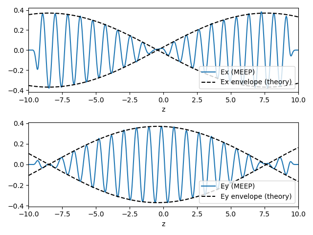
From these expressions, we can calculate the rotation rate $\kappa_c$ at the operating frequency, and hence find the $\mathbf{E}_x$ and $\mathbf{E}_y$ field envelopes for the complex ansatz given at the top of this section.
```python
dfsq = (f0**2 - 1j*fsrc*gamma - fsrc**2)
eperp = epsn + sn * f0**2 * dfsq / (dfsq**2 - (fsrc*b0)**2)
eta = sn * f0**2 * fsrc * b0 / (dfsq**2 - (fsrc*b0)**2)
k_gyro = 2*np.pi*fsrc * np.sqrt(0.5*(eperp - np.sqrt(eperp**2 - eta**2)))
Ex_theory = 0.37 * np.cos(k_gyro * (z - src_z)).real
Ey_theory = 0.37 * np.sin(k_gyro * (z - src_z)).real
plt.figure(2)
plt.subplot(2,1,1)
plt.plot(z, ex_data, label='Ex (MEEP)')
plt.plot(z, Ex_theory, 'k--')
plt.plot(z, -Ex_theory, 'k--', label='Ex envelope (theory)')
plt.xlim(-L/2, L/2); plt.xlabel('z')
plt.legend(loc='lower right')
plt.subplot(2,1,2)
plt.plot(z, ey_data, label='Ey (MEEP)')
plt.plot(z, Ey_theory, 'k--')
plt.plot(z, -Ey_theory, 'k--', label='Ey envelope (theory)')
plt.xlim(-L/2, L/2); plt.xlabel('z')
plt.legend(loc='lower right')
plt.tight_layout()
plt.show()
```
As shown in the figure below, the results are in excellent agreement:
|
