1
2
3
4
5
6
7
8
9
10
11
12
13
14
15
16
17
18
19
20
21
22
23
24
25
26
27
28
29
30
31
32
33
34
35
36
37
38
39
40
41
42
43
44
45
46
47
48
49
50
51
52
53
54
55
56
57
58
59
60
61
62
63
64
65
66
67
68
69
70
71
72
73
74
75
76
77
78
79
80
81
82
83
84
85
86
87
88
89
90
91
92
93
94
95
96
97
98
99
100
101
102
103
104
105
106
107
108
109
110
111
112
113
114
115
116
117
118
119
120
121
122
123
124
125
126
127
128
129
130
131
132
133
134
135
136
137
138
139
140
141
142
143
144
145
146
147
148
149
150
151
152
153
154
155
156
157
158
159
160
161
162
163
164
165
166
167
168
169
170
171
172
173
174
175
176
177
178
179
180
181
182
183
184
185
186
187
188
189
190
191
192
193
194
195
196
197
198
199
200
201
202
203
204
205
206
207
208
209
210
211
|
Hough Line Transform {#tutorial_hough_lines}
====================
Goal
----
In this tutorial you will learn how to:
- Use the OpenCV functions @ref cv::HoughLines and @ref cv::HoughLinesP to detect lines in an
image.
Theory
------
@note The explanation below belongs to the book **Learning OpenCV** by Bradski and Kaehler.
Hough Line Transform
--------------------
-# The Hough Line Transform is a transform used to detect straight lines.
-# To apply the Transform, first an edge detection pre-processing is desirable.
### How does it work?
-# As you know, a line in the image space can be expressed with two variables. For example:
-# In the **Cartesian coordinate system:** Parameters: \f$(m,b)\f$.
-# In the **Polar coordinate system:** Parameters: \f$(r,\theta)\f$

For Hough Transforms, we will express lines in the *Polar system*. Hence, a line equation can be
written as:
\f[y = \left ( -\dfrac{\cos \theta}{\sin \theta} \right ) x + \left ( \dfrac{r}{\sin \theta} \right )\f]
Arranging the terms: \f$r = x \cos \theta + y \sin \theta\f$
-# In general for each point \f$(x_{0}, y_{0})\f$, we can define the family of lines that goes through
that point as:
\f[r_{\theta} = x_{0} \cdot \cos \theta + y_{0} \cdot \sin \theta\f]
Meaning that each pair \f$(r_{\theta},\theta)\f$ represents each line that passes by
\f$(x_{0}, y_{0})\f$.
-# If for a given \f$(x_{0}, y_{0})\f$ we plot the family of lines that goes through it, we get a
sinusoid. For instance, for \f$x_{0} = 8\f$ and \f$y_{0} = 6\f$ we get the following plot (in a plane
\f$\theta\f$ - \f$r\f$):

We consider only points such that \f$r > 0\f$ and \f$0< \theta < 2 \pi\f$.
-# We can do the same operation above for all the points in an image. If the curves of two
different points intersect in the plane \f$\theta\f$ - \f$r\f$, that means that both points belong to a
same line. For instance, following with the example above and drawing the plot for two more
points: \f$x_{1} = 4\f$, \f$y_{1} = 9\f$ and \f$x_{2} = 12\f$, \f$y_{2} = 3\f$, we get:

The three plots intersect in one single point \f$(0.925, 9.6)\f$, these coordinates are the
parameters (\f$\theta, r\f$) or the line in which \f$(x_{0}, y_{0})\f$, \f$(x_{1}, y_{1})\f$ and
\f$(x_{2}, y_{2})\f$ lay.
-# What does all the stuff above mean? It means that in general, a line can be *detected* by
finding the number of intersections between curves.The more curves intersecting means that the
line represented by that intersection have more points. In general, we can define a *threshold*
of the minimum number of intersections needed to *detect* a line.
-# This is what the Hough Line Transform does. It keeps track of the intersection between curves of
every point in the image. If the number of intersections is above some *threshold*, then it
declares it as a line with the parameters \f$(\theta, r_{\theta})\f$ of the intersection point.
### Standard and Probabilistic Hough Line Transform
OpenCV implements two kind of Hough Line Transforms:
a. **The Standard Hough Transform**
- It consists in pretty much what we just explained in the previous section. It gives you as
result a vector of couples \f$(\theta, r_{\theta})\f$
- In OpenCV it is implemented with the function @ref cv::HoughLines
b. **The Probabilistic Hough Line Transform**
- A more efficient implementation of the Hough Line Transform. It gives as output the extremes
of the detected lines \f$(x_{0}, y_{0}, x_{1}, y_{1})\f$
- In OpenCV it is implemented with the function @ref cv::HoughLinesP
Code
----
-# **What does this program do?**
- Loads an image
- Applies either a *Standard Hough Line Transform* or a *Probabilistic Line Transform*.
- Display the original image and the detected line in two windows.
-# The sample code that we will explain can be downloaded from [here](https://github.com/opencv/opencv/tree/master/samples/cpp/houghlines.cpp). A slightly fancier version
(which shows both Hough standard and probabilistic with trackbars for changing the threshold
values) can be found [here](https://github.com/opencv/opencv/tree/master/samples/cpp/tutorial_code/ImgTrans/HoughLines_Demo.cpp).
@include samples/cpp/houghlines.cpp
Explanation
-----------
-# Load an image
@code{.cpp}
Mat src = imread(filename, 0);
if(src.empty())
{
help();
cout << "can not open " << filename << endl;
return -1;
}
@endcode
-# Detect the edges of the image by using a Canny detector
@code{.cpp}
Canny(src, dst, 50, 200, 3);
@endcode
Now we will apply the Hough Line Transform. We will explain how to use both OpenCV functions
available for this purpose:
-# **Standard Hough Line Transform**
-# First, you apply the Transform:
@code{.cpp}
vector<Vec2f> lines;
HoughLines(dst, lines, 1, CV_PI/180, 100, 0, 0 );
@endcode
with the following arguments:
- *dst*: Output of the edge detector. It should be a grayscale image (although in fact it
is a binary one)
- *lines*: A vector that will store the parameters \f$(r,\theta)\f$ of the detected lines
- *rho* : The resolution of the parameter \f$r\f$ in pixels. We use **1** pixel.
- *theta*: The resolution of the parameter \f$\theta\f$ in radians. We use **1 degree**
(CV_PI/180)
- *threshold*: The minimum number of intersections to "*detect*" a line
- *srn* and *stn*: Default parameters to zero. Check OpenCV reference for more info.
-# And then you display the result by drawing the lines.
@code{.cpp}
for( size_t i = 0; i < lines.size(); i++ )
{
float rho = lines[i][0], theta = lines[i][1];
Point pt1, pt2;
double a = cos(theta), b = sin(theta);
double x0 = a*rho, y0 = b*rho;
pt1.x = cvRound(x0 + 1000*(-b));
pt1.y = cvRound(y0 + 1000*(a));
pt2.x = cvRound(x0 - 1000*(-b));
pt2.y = cvRound(y0 - 1000*(a));
line( cdst, pt1, pt2, Scalar(0,0,255), 3, LINE_AA);
}
@endcode
-# **Probabilistic Hough Line Transform**
-# First you apply the transform:
@code{.cpp}
vector<Vec4i> lines;
HoughLinesP(dst, lines, 1, CV_PI/180, 50, 50, 10 );
@endcode
with the arguments:
- *dst*: Output of the edge detector. It should be a grayscale image (although in fact it
is a binary one)
- *lines*: A vector that will store the parameters
\f$(x_{start}, y_{start}, x_{end}, y_{end})\f$ of the detected lines
- *rho* : The resolution of the parameter \f$r\f$ in pixels. We use **1** pixel.
- *theta*: The resolution of the parameter \f$\theta\f$ in radians. We use **1 degree**
(CV_PI/180)
- *threshold*: The minimum number of intersections to "*detect*" a line
- *minLinLength*: The minimum number of points that can form a line. Lines with less than
this number of points are disregarded.
- *maxLineGap*: The maximum gap between two points to be considered in the same line.
-# And then you display the result by drawing the lines.
@code{.cpp}
for( size_t i = 0; i < lines.size(); i++ )
{
Vec4i l = lines[i];
line( cdst, Point(l[0], l[1]), Point(l[2], l[3]), Scalar(0,0,255), 3, LINE_AA);
}
@endcode
-# Display the original image and the detected lines:
@code{.cpp}
imshow("source", src);
imshow("detected lines", cdst);
@endcode
-# Wait until the user exits the program
@code{.cpp}
waitKey();
@endcode
Result
------
@note
The results below are obtained using the slightly fancier version we mentioned in the *Code*
section. It still implements the same stuff as above, only adding the Trackbar for the
Threshold.
Using an input image such as:

We get the following result by using the Probabilistic Hough Line Transform:
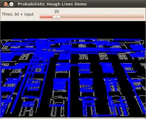
You may observe that the number of lines detected vary while you change the *threshold*. The
explanation is sort of evident: If you establish a higher threshold, fewer lines will be detected
(since you will need more points to declare a line detected).
|
