1
2
3
4
5
6
7
8
9
10
11
12
13
14
15
16
17
18
19
20
21
22
23
24
25
26
27
28
29
30
31
32
33
34
35
36
37
38
39
40
41
42
43
44
45
46
47
48
49
50
51
52
53
54
55
56
57
58
59
60
61
62
63
64
65
66
67
68
69
70
71
72
73
74
75
76
77
78
79
80
81
82
83
84
85
86
87
88
89
90
91
92
93
94
95
96
97
98
99
100
101
102
103
104
105
106
107
108
109
110
111
112
113
114
115
116
117
118
119
120
121
122
123
124
125
126
127
128
129
130
131
132
133
134
135
136
137
138
139
140
141
142
143
144
145
146
147
148
149
150
151
152
153
154
155
156
157
158
159
160
161
162
163
164
165
166
167
168
169
170
171
172
173
174
175
176
177
178
179
180
181
182
183
184
185
186
187
188
189
190
191
|
Support Vector Machines for Non-Linearly Separable Data {#tutorial_non_linear_svms}
=======================================================
Goal
----
In this tutorial you will learn how to:
- Define the optimization problem for SVMs when it is not possible to separate linearly the
training data.
- How to configure the parameters to adapt your SVM for this class of problems.
Motivation
----------
Why is it interesting to extend the SVM optimation problem in order to handle non-linearly separable
training data? Most of the applications in which SVMs are used in computer vision require a more
powerful tool than a simple linear classifier. This stems from the fact that in these tasks __the
training data can be rarely separated using an hyperplane__.
Consider one of these tasks, for example, face detection. The training data in this case is composed
by a set of images that are faces and another set of images that are non-faces (_every other thing
in the world except from faces_). This training data is too complex so as to find a representation
of each sample (_feature vector_) that could make the whole set of faces linearly separable from the
whole set of non-faces.
Extension of the Optimization Problem
-------------------------------------
Remember that using SVMs we obtain a separating hyperplane. Therefore, since the training data is
now non-linearly separable, we must admit that the hyperplane found will misclassify some of the
samples. This _misclassification_ is a new variable in the optimization that must be taken into
account. The new model has to include both the old requirement of finding the hyperplane that gives
the biggest margin and the new one of generalizing the training data correctly by not allowing too
many classification errors.
We start here from the formulation of the optimization problem of finding the hyperplane which
maximizes the __margin__ (this is explained in the previous tutorial (@ref tutorial_introduction_to_svm):
\f[\min_{\beta, \beta_{0}} L(\beta) = \frac{1}{2}||\beta||^{2} \text{ subject to } y_{i}(\beta^{T} x_{i} + \beta_{0}) \geq 1 \text{ } \forall i\f]
There are multiple ways in which this model can be modified so it takes into account the
misclassification errors. For example, one could think of minimizing the same quantity plus a
constant times the number of misclassification errors in the training data, i.e.:
\f[\min ||\beta||^{2} + C \text{(\# misclassication errors)}\f]
However, this one is not a very good solution since, among some other reasons, we do not distinguish
between samples that are misclassified with a small distance to their appropriate decision region or
samples that are not. Therefore, a better solution will take into account the _distance of the
misclassified samples to their correct decision regions_, i.e.:
\f[\min ||\beta||^{2} + C \text{(distance of misclassified samples to their correct regions)}\f]
For each sample of the training data a new parameter \f$\xi_{i}\f$ is defined. Each one of these
parameters contains the distance from its corresponding training sample to their correct decision
region. The following picture shows non-linearly separable training data from two classes, a
separating hyperplane and the distances to their correct regions of the samples that are
misclassified.
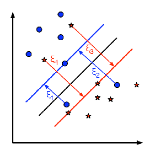
@note Only the distances of the samples that are misclassified are shown in the picture. The
distances of the rest of the samples are zero since they lay already in their correct decision
region.
The red and blue lines that appear on the picture are the margins to each one of the
decision regions. It is very __important__ to realize that each of the \f$\xi_{i}\f$ goes from a
misclassified training sample to the margin of its appropriate region.
Finally, the new formulation for the optimization problem is:
\f[\min_{\beta, \beta_{0}} L(\beta) = ||\beta||^{2} + C \sum_{i} {\xi_{i}} \text{ subject to } y_{i}(\beta^{T} x_{i} + \beta_{0}) \geq 1 - \xi_{i} \text{ and } \xi_{i} \geq 0 \text{ } \forall i\f]
How should the parameter C be chosen? It is obvious that the answer to this question depends on how
the training data is distributed. Although there is no general answer, it is useful to take into
account these rules:
- Large values of C give solutions with _less misclassification errors_ but a _smaller margin_.
Consider that in this case it is expensive to make misclassification errors. Since the aim of
the optimization is to minimize the argument, few misclassifications errors are allowed.
- Small values of C give solutions with _bigger margin_ and _more classification errors_. In this
case the minimization does not consider that much the term of the sum so it focuses more on
finding a hyperplane with big margin.
Source Code
-----------
You may also find the source code in `samples/cpp/tutorial_code/ml/non_linear_svms` folder of the OpenCV source library or
[download it from here](https://github.com/opencv/tree/master/samples/cpp/tutorial_code/ml/non_linear_svms/non_linear_svms.cpp).
@note The following code has been implemented with OpenCV 3.0 classes and functions. An equivalent version of the code
using OpenCV 2.4 can be found in [this page.](http://docs.opencv.org/2.4/doc/tutorials/ml/non_linear_svms/non_linear_svms.html#nonlinearsvms)
@include cpp/tutorial_code/ml/non_linear_svms/non_linear_svms.cpp
Explanation
-----------
-# __Set up the training data__
The training data of this exercise is formed by a set of labeled 2D-points that belong to one of
two different classes. To make the exercise more appealing, the training data is generated
randomly using a uniform probability density functions (PDFs).
We have divided the generation of the training data into two main parts.
In the first part we generate data for both classes that is linearly separable.
@snippet cpp/tutorial_code/ml/non_linear_svms/non_linear_svms.cpp setup1
In the second part we create data for both classes that is non-linearly separable, data that
overlaps.
@snippet cpp/tutorial_code/ml/non_linear_svms/non_linear_svms.cpp setup2
-# __Set up SVM's parameters__
@note In the previous tutorial @ref tutorial_introduction_to_svm there is an explanation of the
atributes of the class @ref cv::ml::SVM that we configure here before training the SVM.
@snippet cpp/tutorial_code/ml/non_linear_svms/non_linear_svms.cpp init
There are just two differences between the configuration we do here and the one that was done in
the previous tutorial (@ref tutorial_introduction_to_svm) that we use as reference.
- _C_. We chose here a small value of this parameter in order not to punish too much the
misclassification errors in the optimization. The idea of doing this stems from the will of
obtaining a solution close to the one intuitively expected. However, we recommend to get a
better insight of the problem by making adjustments to this parameter.
@note In this case there are just very few points in the overlapping region between classes.
By giving a smaller value to __FRAC_LINEAR_SEP__ the density of points can be incremented and the
impact of the parameter _C_ explored deeply.
- _Termination Criteria of the algorithm_. The maximum number of iterations has to be
increased considerably in order to solve correctly a problem with non-linearly separable
training data. In particular, we have increased in five orders of magnitude this value.
-# __Train the SVM__
We call the method @ref cv::ml::SVM::train to build the SVM model. Watch out that the training
process may take a quite long time. Have patiance when your run the program.
@snippet cpp/tutorial_code/ml/non_linear_svms/non_linear_svms.cpp train
-# __Show the Decision Regions__
The method @ref cv::ml::SVM::predict is used to classify an input sample using a trained SVM. In
this example we have used this method in order to color the space depending on the prediction done
by the SVM. In other words, an image is traversed interpreting its pixels as points of the
Cartesian plane. Each of the points is colored depending on the class predicted by the SVM; in
dark green if it is the class with label 1 and in dark blue if it is the class with label 2.
@snippet cpp/tutorial_code/ml/non_linear_svms/non_linear_svms.cpp show
-# __Show the training data__
The method @ref cv::circle is used to show the samples that compose the training data. The samples
of the class labeled with 1 are shown in light green and in light blue the samples of the class
labeled with 2.
@snippet cpp/tutorial_code/ml/non_linear_svms/non_linear_svms.cpp show_data
-# __Support vectors__
We use here a couple of methods to obtain information about the support vectors. The method
@ref cv::ml::SVM::getSupportVectors obtain all support vectors. We have used this methods here
to find the training examples that are support vectors and highlight them.
@snippet cpp/tutorial_code/ml/non_linear_svms/non_linear_svms.cpp show_vectors
Results
-------
- The code opens an image and shows the training examples of both classes. The points of one class
are represented with light green and light blue ones are used for the other class.
- The SVM is trained and used to classify all the pixels of the image. This results in a division
of the image in a blue region and a green region. The boundary between both regions is the
separating hyperplane. Since the training data is non-linearly separable, it can be seen that
some of the examples of both classes are misclassified; some green points lay on the blue region
and some blue points lay on the green one.
- Finally the support vectors are shown using gray rings around the training examples.

You may observe a runtime instance of this on the [YouTube here](https://www.youtube.com/watch?v=vFv2yPcSo-Q).
\htmlonly
<div align="center">
<iframe title="Support Vector Machines for Non-Linearly Separable Data" width="560" height="349" src="http://www.youtube.com/embed/vFv2yPcSo-Q?rel=0&loop=1" frameborder="0" allowfullscreen align="middle"></iframe>
</div>
\endhtmlonly
|
