Image Thresholding {#tutorial_py_thresholding}
==================

Goal
----

-   In this tutorial, you will learn simple thresholding, adaptive thresholding and Otsu's thresholding.
-   You will learn the functions **cv.threshold** and **cv.adaptiveThreshold**.

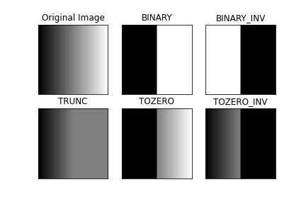
Simple Thresholding
-------------------

Here, the matter is straight-forward. For every pixel, the same threshold value is applied.
If the pixel value is smaller than the threshold, it is set to 0, otherwise it is set to a maximum value.
The function **cv.threshold** is used to apply the thresholding.
The first argument is the source image, which **should be a grayscale image**.
The second argument is the threshold value which is used to classify the pixel values.
The third argument is the maximum value which is assigned to pixel values exceeding the threshold.
OpenCV provides different types of thresholding which is given by the fourth parameter of the function.
Basic thresholding as described above is done by using the type cv.THRESH_BINARY.
All simple thresholding types are:

-   cv.THRESH_BINARY
-   cv.THRESH_BINARY_INV
-   cv.THRESH_TRUNC
-   cv.THRESH_TOZERO
-   cv.THRESH_TOZERO_INV

See the documentation of the types for the differences.

The method returns two outputs.
The first is the threshold that was used and the second output is the **thresholded image**.

This code compares the different simple thresholding types:
@code{.py}
import cv2 as cv
import numpy as np
from matplotlib import pyplot as plt

img = cv.imread('gradient.png',0)
ret,thresh1 = cv.threshold(img,127,255,cv.THRESH_BINARY)
ret,thresh2 = cv.threshold(img,127,255,cv.THRESH_BINARY_INV)
ret,thresh3 = cv.threshold(img,127,255,cv.THRESH_TRUNC)
ret,thresh4 = cv.threshold(img,127,255,cv.THRESH_TOZERO)
ret,thresh5 = cv.threshold(img,127,255,cv.THRESH_TOZERO_INV)

titles = ['Original Image','BINARY','BINARY_INV','TRUNC','TOZERO','TOZERO_INV']
images = [img, thresh1, thresh2, thresh3, thresh4, thresh5]

for i in range(6):
    plt.subplot(2,3,i+1),plt.imshow(images[i],'gray',vmin=0,vmax=255)
    plt.title(titles[i])
    plt.xticks([]),plt.yticks([])

plt.show()
@endcode
@note To plot multiple images, we have used the plt.subplot() function. Please checkout the matplotlib docs for more details.

The code yields this result:

![image](images/threshold.jpg)

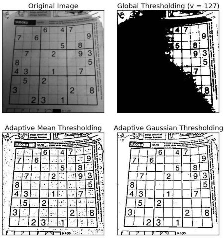
Adaptive Thresholding
---------------------

In the previous section, we used one global value as a threshold.
But this might not be good in all cases, e.g. if an image has different lighting conditions in different areas.
In that case, adaptive thresholding can help.
Here, the algorithm determines the threshold for a pixel based on a small region around it.
So we get different thresholds for different regions of the same image which gives better results for images with varying illumination.

In addition to the parameters described above, the method cv.adaptiveThreshold takes three input parameters:

The **adaptiveMethod** decides how the threshold value is calculated:
    -   cv.ADAPTIVE_THRESH_MEAN_C: The threshold value is the mean of the neighbourhood area minus the constant **C**.
    -   cv.ADAPTIVE_THRESH_GAUSSIAN_C: The threshold value is a gaussian-weighted sum of the neighbourhood
        values minus the constant **C**.

The **blockSize** determines the size of the neighbourhood area and **C** is a constant that is subtracted from the mean or weighted sum of the neighbourhood pixels.

The code below compares global thresholding and adaptive thresholding for an image with varying
illumination:
@code{.py}
import cv2 as cv
import numpy as np
from matplotlib import pyplot as plt

img = cv.imread('sudoku.png',0)
img = cv.medianBlur(img,5)

ret,th1 = cv.threshold(img,127,255,cv.THRESH_BINARY)
th2 = cv.adaptiveThreshold(img,255,cv.ADAPTIVE_THRESH_MEAN_C,\
            cv.THRESH_BINARY,11,2)
th3 = cv.adaptiveThreshold(img,255,cv.ADAPTIVE_THRESH_GAUSSIAN_C,\
            cv.THRESH_BINARY,11,2)

titles = ['Original Image', 'Global Thresholding (v = 127)',
            'Adaptive Mean Thresholding', 'Adaptive Gaussian Thresholding']
images = [img, th1, th2, th3]

for i in range(4):
    plt.subplot(2,2,i+1),plt.imshow(images[i],'gray')
    plt.title(titles[i])
    plt.xticks([]),plt.yticks([])
plt.show()
@endcode
Result:

![image](images/ada_threshold.jpg)

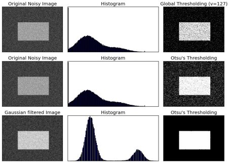
Otsu's Binarization
-------------------

In global thresholding, we used an arbitrary chosen value as a threshold.
In contrast, Otsu's method avoids having to choose a value and determines it automatically.

Consider an image with only two distinct image values (*bimodal image*), where the histogram would only consist of two peaks.
A good threshold would be in the middle of those two values.
Similarly, Otsu's method determines an optimal global threshold value from the image histogram.

In order to do so, the cv.threshold() function is used, where cv.THRESH_OTSU is passed as an extra flag.
The threshold value can be chosen arbitrary.
The algorithm then finds the optimal threshold value which is returned as the first output.

Check out the example below.
The input image is a noisy image.
In the first case, global thresholding with a value of 127 is applied.
In the second case, Otsu's thresholding is applied directly.
In the third case, the image is first filtered with a 5x5 gaussian kernel to remove the noise, then Otsu thresholding is applied.
See how noise filtering improves the result.
@code{.py}
import cv2 as cv
import numpy as np
from matplotlib import pyplot as plt

img = cv.imread('noisy2.png',0)

# global thresholding
ret1,th1 = cv.threshold(img,127,255,cv.THRESH_BINARY)

# Otsu's thresholding
ret2,th2 = cv.threshold(img,0,255,cv.THRESH_BINARY+cv.THRESH_OTSU)

# Otsu's thresholding after Gaussian filtering
blur = cv.GaussianBlur(img,(5,5),0)
ret3,th3 = cv.threshold(blur,0,255,cv.THRESH_BINARY+cv.THRESH_OTSU)

# plot all the images and their histograms
images = [img, 0, th1,
          img, 0, th2,
          blur, 0, th3]
titles = ['Original Noisy Image','Histogram','Global Thresholding (v=127)',
          'Original Noisy Image','Histogram',"Otsu's Thresholding",
          'Gaussian filtered Image','Histogram',"Otsu's Thresholding"]

for i in range(3):
    plt.subplot(3,3,i*3+1),plt.imshow(images[i*3],'gray')
    plt.title(titles[i*3]), plt.xticks([]), plt.yticks([])
    plt.subplot(3,3,i*3+2),plt.hist(images[i*3].ravel(),256)
    plt.title(titles[i*3+1]), plt.xticks([]), plt.yticks([])
    plt.subplot(3,3,i*3+3),plt.imshow(images[i*3+2],'gray')
    plt.title(titles[i*3+2]), plt.xticks([]), plt.yticks([])
plt.show()
@endcode
Result:

![image](images/otsu.jpg)

### How does Otsu's Binarization work?

This section demonstrates a Python implementation of Otsu's binarization to show how it actually
works. If you are not interested, you can skip this.

Since we are working with bimodal images, Otsu's algorithm tries to find a threshold value (t) which
minimizes the **weighted within-class variance** given by the relation:

\f[\sigma_w^2(t) = q_1(t)\sigma_1^2(t)+q_2(t)\sigma_2^2(t)\f]

where

\f[q_1(t) = \sum_{i=1}^{t} P(i) \quad \& \quad q_2(t) = \sum_{i=t+1}^{I} P(i)\f]\f[\mu_1(t) = \sum_{i=1}^{t} \frac{iP(i)}{q_1(t)} \quad \& \quad \mu_2(t) = \sum_{i=t+1}^{I} \frac{iP(i)}{q_2(t)}\f]\f[\sigma_1^2(t) = \sum_{i=1}^{t} [i-\mu_1(t)]^2 \frac{P(i)}{q_1(t)} \quad \& \quad \sigma_2^2(t) = \sum_{i=t+1}^{I} [i-\mu_2(t)]^2 \frac{P(i)}{q_2(t)}\f]

It actually finds a value of t which lies in between two peaks such that variances to both classes
are minimal. It can be simply implemented in Python as follows:
@code{.py}
img = cv.imread('noisy2.png',0)
blur = cv.GaussianBlur(img,(5,5),0)

# find normalized_histogram, and its cumulative distribution function
hist = cv.calcHist([blur],[0],None,[256],[0,256])
hist_norm = hist.ravel()/hist.sum()
Q = hist_norm.cumsum()

bins = np.arange(256)

fn_min = np.inf
thresh = -1

for i in range(1,256):
    p1,p2 = np.hsplit(hist_norm,[i]) # probabilities
    q1,q2 = Q[i],Q[255]-Q[i] # cum sum of classes
    if q1 < 1.e-6 or q2 < 1.e-6:
        continue
    b1,b2 = np.hsplit(bins,[i]) # weights

    # finding means and variances
    m1,m2 = np.sum(p1*b1)/q1, np.sum(p2*b2)/q2
    v1,v2 = np.sum(((b1-m1)**2)*p1)/q1,np.sum(((b2-m2)**2)*p2)/q2

    # calculates the minimization function
    fn = v1*q1 + v2*q2
    if fn < fn_min:
        fn_min = fn
        thresh = i

# find otsu's threshold value with OpenCV function
ret, otsu = cv.threshold(blur,0,255,cv.THRESH_BINARY+cv.THRESH_OTSU)
print( "{} {}".format(thresh,ret) )
@endcode

Additional Resources
--------------------

-#  Digital Image Processing, Rafael C. Gonzalez

Exercises
---------

-#  There are some optimizations available for Otsu's binarization. You can search and implement it.