Basic concepts of the homography explained with code {#tutorial_homography}
====================================================

@tableofcontents

@prev_tutorial{tutorial_akaze_tracking}

|    |    |
| -: | :- |
| Compatibility | OpenCV >= 3.0 |

@tableofcontents

Introduction {#tutorial_homography_Introduction}
============

This tutorial will demonstrate the basic concepts of the homography with some codes.
For detailed explanations about the theory, please refer to a computer vision course or a computer vision book, e.g.:
*   Multiple View Geometry in Computer Vision, @cite HartleyZ00.
*   An Invitation to 3-D Vision: From Images to Geometric Models, @cite Ma:2003:IVI
*   Computer Vision: Algorithms and Applications, @cite RS10

The tutorial code can be found here [C++](https://github.com/opencv/opencv/tree/4.x/samples/cpp/tutorial_code/features2D/Homography),
[Python](https://github.com/opencv/opencv/tree/4.x/samples/python/tutorial_code/features2D/Homography),
[Java](https://github.com/opencv/opencv/tree/4.x/samples/java/tutorial_code/features2D/Homography).
The images used in this tutorial can be found [here](https://github.com/opencv/opencv/tree/4.x/samples/data) (`left*.jpg`).

Basic theory {#tutorial_homography_Basic_theory}
------------

### What is the homography matrix? {#tutorial_homography_What_is_the_homography_matrix}

Briefly, the planar homography relates the transformation between two planes (up to a scale factor):

\f[
  s
  \begin{bmatrix}
  x^{'} \\
  y^{'} \\
  1
  \end{bmatrix} = H
  \begin{bmatrix}
  x \\
  y \\
  1
  \end{bmatrix} =
  \begin{bmatrix}
  h_{11} & h_{12} & h_{13} \\
  h_{21} & h_{22} & h_{23} \\
  h_{31} & h_{32} & h_{33}
  \end{bmatrix}
  \begin{bmatrix}
  x \\
  y \\
  1
  \end{bmatrix}
\f]

The homography matrix is a `3x3` matrix but with 8 DoF (degrees of freedom) as it is estimated up to a scale. It is generally normalized (see also \ref lecture_16 "1")
with \f$ h_{33} = 1 \f$ or \f$ h_{11}^2 + h_{12}^2 + h_{13}^2 + h_{21}^2 + h_{22}^2 + h_{23}^2 + h_{31}^2 + h_{32}^2 + h_{33}^2 = 1 \f$.

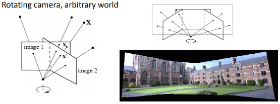
The following examples show different kinds of transformation but all relate a transformation between two planes.

*   a planar surface and the image plane (image taken from \ref projective_transformations "2")

![](images/homography_transformation_example1.jpg)

*   a planar surface viewed by two camera positions (images taken from \ref szeliski "3" and \ref projective_transformations "2")

![](images/homography_transformation_example2.jpg)

*   a rotating camera around its axis of projection, equivalent to consider that the points are on a plane at infinity (image taken from \ref projective_transformations "2")

![](images/homography_transformation_example3.jpg)

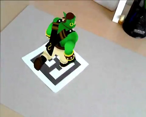
### How the homography transformation can be useful? {#tutorial_homography_How_the_homography_transformation_can_be_useful}

*   Camera pose estimation from coplanar points for augmented reality with marker for instance (see the previous first example)

![](images/homography_pose_estimation.jpg)

*   Perspective removal / correction (see the previous second example)

![](images/homography_perspective_correction.jpg)

*   Panorama stitching (see the previous second and third example)

![](images/homography_panorama_stitching.jpg)

Demonstration codes {#tutorial_homography_Demonstration_codes}
-------------------

### Demo 1: Pose estimation from coplanar points {#tutorial_homography_Demo1}

\note Please note that the code to estimate the camera pose from the homography is an example and you should use instead @ref cv::solvePnP if you want to estimate the camera pose for a planar or an arbitrary object.

The homography can be estimated using for instance the Direct Linear Transform (DLT) algorithm (see \ref lecture_16 "1" for more information).
As the object is planar, the transformation between points expressed in the object frame and projected points into the image plane expressed in the normalized camera frame is a homography. Only because the object is planar,
the camera pose can be retrieved from the homography, assuming the camera intrinsic parameters are known (see \ref projective_transformations "2" or \ref answer_dsp "4").
This can be tested easily using a chessboard object and `findChessboardCorners()` to get the corner locations in the image.

The first thing consists to detect the chessboard corners, the chessboard size (`patternSize`), here `9x6`, is required:

@snippet pose_from_homography.cpp find-chessboard-corners

![](images/homography_pose_chessboard_corners.jpg)

The object points expressed in the object frame can be computed easily knowing the size of a chessboard square:

@snippet pose_from_homography.cpp compute-chessboard-object-points

The coordinate `Z=0` must be removed for the homography estimation part:

@snippet pose_from_homography.cpp compute-object-points

The image points expressed in the normalized camera can be computed from the corner points and by applying a reverse perspective transformation using the camera intrinsics and the distortion coefficients:

@snippet pose_from_homography.cpp load-intrinsics

@snippet pose_from_homography.cpp compute-image-points

The homography can then be estimated with:

@snippet pose_from_homography.cpp estimate-homography

A quick solution to retrieve the pose from the homography matrix is (see \ref pose_ar "5"):

@snippet pose_from_homography.cpp pose-from-homography

\f[
  \begin{align*}
  \boldsymbol{X} &= \left( X, Y, 0, 1 \right ) \\
  \boldsymbol{x} &= \boldsymbol{P}\boldsymbol{X} \\
                 &= \boldsymbol{K} \left[ \boldsymbol{r_1} \hspace{0.5em} \boldsymbol{r_2} \hspace{0.5em} \boldsymbol{r_3} \hspace{0.5em} \boldsymbol{t} \right ]
  \begin{pmatrix}
  X \\
  Y \\
  0 \\
  1
  \end{pmatrix} \\
             &= \boldsymbol{K} \left[ \boldsymbol{r_1} \hspace{0.5em} \boldsymbol{r_2} \hspace{0.5em} \boldsymbol{t} \right ]
  \begin{pmatrix}
  X \\
  Y \\
  1
  \end{pmatrix} \\
  &= \boldsymbol{H}
  \begin{pmatrix}
  X \\
  Y \\
  1
  \end{pmatrix}
  \end{align*}
\f]

\f[
  \begin{align*}
  \boldsymbol{H} &= \lambda \boldsymbol{K} \left[ \boldsymbol{r_1} \hspace{0.5em} \boldsymbol{r_2} \hspace{0.5em} \boldsymbol{t} \right ] \\
  \boldsymbol{K}^{-1} \boldsymbol{H} &= \lambda \left[ \boldsymbol{r_1} \hspace{0.5em} \boldsymbol{r_2} \hspace{0.5em} \boldsymbol{t} \right ] \\
  \boldsymbol{P} &= \boldsymbol{K} \left[ \boldsymbol{r_1} \hspace{0.5em} \boldsymbol{r_2} \hspace{0.5em} \left( \boldsymbol{r_1} \times \boldsymbol{r_2} \right ) \hspace{0.5em} \boldsymbol{t} \right ]
  \end{align*}
\f]

This is a quick solution (see also \ref projective_transformations "2") as this does not ensure that the resulting rotation matrix will be orthogonal and the scale is estimated roughly by normalize the first column to 1.

A solution to have a proper rotation matrix (with the properties of a rotation matrix) consists to apply a polar decomposition
(see \ref polar_decomposition "6" or \ref polar_decomposition_svd "7" for some information):

@snippet pose_from_homography.cpp polar-decomposition-of-the-rotation-matrix

To check the result, the object frame projected into the image with the estimated camera pose is displayed:

![](images/homography_pose.jpg)

### Demo 2: Perspective correction {#tutorial_homography_Demo2}

In this example, a source image will be transformed into a desired perspective view by computing the homography that maps the source points into the desired points.
The following image shows the source image (left) and the chessboard view that we want to transform into the desired chessboard view (right).

![Source and desired views](images/homography_source_desired_images.jpg)

The first step consists to detect the chessboard corners in the source and desired images:

@add_toggle_cpp
@snippet perspective_correction.cpp find-corners
@end_toggle

@add_toggle_python
@snippet samples/python/tutorial_code/features2D/Homography/perspective_correction.py find-corners
@end_toggle

@add_toggle_java
@snippet samples/java/tutorial_code/features2D/Homography/PerspectiveCorrection.java find-corners
@end_toggle

The homography is estimated easily with:

@add_toggle_cpp
@snippet perspective_correction.cpp estimate-homography
@end_toggle

@add_toggle_python
@snippet samples/python/tutorial_code/features2D/Homography/perspective_correction.py estimate-homography
@end_toggle

@add_toggle_java
@snippet samples/java/tutorial_code/features2D/Homography/PerspectiveCorrection.java estimate-homography
@end_toggle

To warp the source chessboard view into the desired chessboard view, we use @ref cv::warpPerspective

@add_toggle_cpp
@snippet perspective_correction.cpp warp-chessboard
@end_toggle

@add_toggle_python
@snippet samples/python/tutorial_code/features2D/Homography/perspective_correction.py warp-chessboard
@end_toggle

@add_toggle_java
@snippet samples/java/tutorial_code/features2D/Homography/PerspectiveCorrection.java warp-chessboard
@end_toggle

The result image is:

![](images/homography_perspective_correction_chessboard_warp.jpg)

To compute the coordinates of the source corners transformed by the homography:

@add_toggle_cpp
@snippet perspective_correction.cpp compute-transformed-corners
@end_toggle

@add_toggle_python
@snippet samples/python/tutorial_code/features2D/Homography/perspective_correction.py compute-transformed-corners
@end_toggle

@add_toggle_java
@snippet samples/java/tutorial_code/features2D/Homography/PerspectiveCorrection.java compute-transformed-corners
@end_toggle

To check the correctness of the calculation, the matching lines are displayed:

![](images/homography_perspective_correction_chessboard_matches.jpg)

### Demo 3: Homography from the camera displacement {#tutorial_homography_Demo3}

The homography relates the transformation between two planes and it is possible to retrieve the corresponding camera displacement that allows to go from the first to the second plane view (see @cite Malis for more information).
Before going into the details that allow to compute the homography from the camera displacement, some recalls about camera pose and homogeneous transformation.

The function @ref cv::solvePnP allows to compute the camera pose from the correspondences 3D object points (points expressed in the object frame) and the projected 2D image points (object points viewed in the image).
The intrinsic parameters and the distortion coefficients are required (see the camera calibration process).

\f[
  \begin{align*}
  s
  \begin{bmatrix}
  u \\
  v \\
  1
  \end{bmatrix} &=
  \begin{bmatrix}
  f_x & 0 & c_x \\
  0 & f_y & c_y \\
  0 & 0 & 1
  \end{bmatrix}
  \begin{bmatrix}
  r_{11} & r_{12} & r_{13} & t_x \\
  r_{21} & r_{22} & r_{23} & t_y \\
  r_{31} & r_{32} & r_{33} & t_z
  \end{bmatrix}
  \begin{bmatrix}
  X_o \\
  Y_o \\
  Z_o \\
  1
  \end{bmatrix} \\
  &= \boldsymbol{K} \hspace{0.2em} ^{c}\textrm{M}_o
  \begin{bmatrix}
  X_o \\
  Y_o \\
  Z_o \\
  1
  \end{bmatrix}
  \end{align*}
\f]

\f$ \boldsymbol{K} \f$ is the intrinsic matrix and \f$ ^{c}\textrm{M}_o \f$ is the camera pose. The output of @ref cv::solvePnP is exactly this: `rvec` is the Rodrigues rotation vector and `tvec` the translation vector.

\f$ ^{c}\textrm{M}_o \f$ can be represented in a homogeneous form and allows to transform a point expressed in the object frame into the camera frame:

\f[
  \begin{align*}
  \begin{bmatrix}
  X_c \\
  Y_c \\
  Z_c \\
  1
  \end{bmatrix} &=
  \hspace{0.2em} ^{c}\textrm{M}_o
  \begin{bmatrix}
  X_o \\
  Y_o \\
  Z_o \\
  1
  \end{bmatrix} \\
  &=
  \begin{bmatrix}
  ^{c}\textrm{R}_o & ^{c}\textrm{t}_o \\
  0_{1\times3} & 1
  \end{bmatrix}
  \begin{bmatrix}
  X_o \\
  Y_o \\
  Z_o \\
  1
  \end{bmatrix} \\
  &=
  \begin{bmatrix}
  r_{11} & r_{12} & r_{13} & t_x \\
  r_{21} & r_{22} & r_{23} & t_y \\
  r_{31} & r_{32} & r_{33} & t_z \\
  0 & 0 & 0 & 1
  \end{bmatrix}
  \begin{bmatrix}
  X_o \\
  Y_o \\
  Z_o \\
  1
  \end{bmatrix}
  \end{align*}
\f]

Transform a point expressed in one frame to another frame can be easily done with matrix multiplication:

*   \f$ ^{c_1}\textrm{M}_o \f$ is the camera pose for the camera 1
*   \f$ ^{c_2}\textrm{M}_o \f$ is the camera pose for the camera 2

To transform a 3D point expressed in the camera 1 frame to the camera 2 frame:

\f[
  ^{c_2}\textrm{M}_{c_1} = \hspace{0.2em} ^{c_2}\textrm{M}_{o} \cdot \hspace{0.1em} ^{o}\textrm{M}_{c_1} = \hspace{0.2em} ^{c_2}\textrm{M}_{o} \cdot \hspace{0.1em} \left( ^{c_1}\textrm{M}_{o} \right )^{-1} =
  \begin{bmatrix}
  ^{c_2}\textrm{R}_{o} & ^{c_2}\textrm{t}_{o} \\
  0_{3 \times 1} & 1
  \end{bmatrix} \cdot
  \begin{bmatrix}
  ^{c_1}\textrm{R}_{o}^T & - \hspace{0.2em} ^{c_1}\textrm{R}_{o}^T \cdot \hspace{0.2em} ^{c_1}\textrm{t}_{o} \\
  0_{1 \times 3} & 1
  \end{bmatrix}
\f]

In this example, we will compute the camera displacement between two camera poses with respect to the chessboard object. The first step consists to compute the camera poses for the two images:

@snippet homography_from_camera_displacement.cpp compute-poses

![](images/homography_camera_displacement_poses.jpg)

The camera displacement can be computed from the camera poses using the formulas above:

@snippet homography_from_camera_displacement.cpp compute-c2Mc1

The homography related to a specific plane computed from the camera displacement is:

![By Homography-transl.svg: Per Rosengren derivative work: Appoose (Homography-transl.svg) [CC BY 3.0 (http://creativecommons.org/licenses/by/3.0)], via Wikimedia Commons](images/homography_camera_displacement.png)

On this figure, `n` is the normal vector of the plane and `d` the distance between the camera frame and the plane along the plane normal.
The [equation](https://en.wikipedia.org/wiki/Homography_(computer_vision)#3D_plane_to_plane_equation) to compute the homography from the camera displacement is:

\f[
  ^{2}\textrm{H}_{1} = \hspace{0.2em} ^{2}\textrm{R}_{1} - \hspace{0.1em} \frac{^{2}\textrm{t}_{1} \cdot n^T}{d}
\f]

Where \f$ ^{2}\textrm{H}_{1} \f$ is the homography matrix that maps the points in the first camera frame to the corresponding points in the second camera frame, \f$ ^{2}\textrm{R}_{1} = \hspace{0.2em} ^{c_2}\textrm{R}_{o} \cdot \hspace{0.1em} ^{c_1}\textrm{R}_{o}^{T} \f$
is the rotation matrix that represents the rotation between the two camera frames and \f$ ^{2}\textrm{t}_{1} = \hspace{0.2em} ^{c_2}\textrm{R}_{o} \cdot \left( - \hspace{0.1em} ^{c_1}\textrm{R}_{o}^{T} \cdot \hspace{0.1em} ^{c_1}\textrm{t}_{o} \right ) + \hspace{0.1em} ^{c_2}\textrm{t}_{o} \f$
the translation vector between the two camera frames.

Here the normal vector `n` is the plane normal expressed in the camera frame 1 and can be computed as the cross product of 2 vectors (using 3 non collinear points that lie on the plane) or in our case directly with:

@snippet homography_from_camera_displacement.cpp compute-plane-normal-at-camera-pose-1

The distance `d` can be computed as the dot product between the plane normal and a point on the plane or by computing the [plane equation](http://mathworld.wolfram.com/Plane.html) and using the D coefficient:

@snippet homography_from_camera_displacement.cpp compute-plane-distance-to-the-camera-frame-1

The projective homography matrix \f$ \textbf{G} \f$ can be computed from the Euclidean homography \f$ \textbf{H} \f$ using the intrinsic matrix \f$ \textbf{K} \f$ (see @cite Malis), here assuming the same camera between the two plane views:

\f[
  \textbf{G} = \gamma \textbf{K} \textbf{H} \textbf{K}^{-1}
\f]

@snippet homography_from_camera_displacement.cpp compute-homography

In our case, the Z-axis of the chessboard goes inside the object whereas in the homography figure it goes outside. This is just a matter of sign:

\f[
  ^{2}\textrm{H}_{1} = \hspace{0.2em} ^{2}\textrm{R}_{1} + \hspace{0.1em} \frac{^{2}\textrm{t}_{1} \cdot n^T}{d}
\f]

@snippet homography_from_camera_displacement.cpp compute-homography-from-camera-displacement

We will now compare the projective homography computed from the camera displacement with the one estimated with @ref cv::findHomography

```
findHomography H:
[0.32903393332201, -1.244138808862929, 536.4769088231476;
 0.6969763913334046, -0.08935909072571542, -80.34068504082403;
 0.00040511729592961, -0.001079740100565013, 0.9999999999999999]

homography from camera displacement:
[0.4160569997384721, -1.306889006892538, 553.7055461075881;
 0.7917584252773352, -0.06341244158456338, -108.2770029401219;
 0.0005926357240956578, -0.001020651672127799, 1]

```

The homography matrices are similar. If we compare the image 1 warped using both homography matrices:

![Left: image warped using the homography estimated. Right: using the homography computed from the camera displacement](images/homography_camera_displacement_compare.jpg)

Visually, it is hard to distinguish a difference between the result image from the homography computed from the camera displacement and the one estimated with @ref cv::findHomography function.

### Demo 4: Decompose the homography matrix {#tutorial_homography_Demo4}

OpenCV 3 contains the function @ref cv::decomposeHomographyMat which allows to decompose the homography matrix to a set of rotations, translations and plane normals.
First we will decompose the homography matrix computed from the camera displacement:

@snippet decompose_homography.cpp compute-homography-from-camera-displacement

The results of @ref cv::decomposeHomographyMat are:

@snippet decompose_homography.cpp decompose-homography-from-camera-displacement

```
Solution 0:
rvec from homography decomposition: [-0.0919829920641369, -0.5372581036567992, 1.310868863540717]
rvec from camera displacement: [-0.09198299206413783, -0.5372581036567995, 1.310868863540717]
tvec from homography decomposition: [-0.7747961019053186, -0.02751124463434032, -0.6791980037590677] and scaled by d: [-0.1578091561210742, -0.005603443652993778, -0.1383378976078466]
tvec from camera displacement: [0.1578091561210745, 0.005603443652993617, 0.1383378976078466]
plane normal from homography decomposition: [-0.1973513139420648, 0.6283451996579074, -0.7524857267431757]
plane normal at camera 1 pose: [0.1973513139420654, -0.6283451996579068, 0.752485726743176]

Solution 1:
rvec from homography decomposition: [-0.0919829920641369, -0.5372581036567992, 1.310868863540717]
rvec from camera displacement: [-0.09198299206413783, -0.5372581036567995, 1.310868863540717]
tvec from homography decomposition: [0.7747961019053186, 0.02751124463434032, 0.6791980037590677] and scaled by d: [0.1578091561210742, 0.005603443652993778, 0.1383378976078466]
tvec from camera displacement: [0.1578091561210745, 0.005603443652993617, 0.1383378976078466]
plane normal from homography decomposition: [0.1973513139420648, -0.6283451996579074, 0.7524857267431757]
plane normal at camera 1 pose: [0.1973513139420654, -0.6283451996579068, 0.752485726743176]

Solution 2:
rvec from homography decomposition: [0.1053487907109967, -0.1561929144786397, 1.401356552358475]
rvec from camera displacement: [-0.09198299206413783, -0.5372581036567995, 1.310868863540717]
tvec from homography decomposition: [-0.4666552552894618, 0.1050032934770042, -0.913007654671646] and scaled by d: [-0.0950475510338766, 0.02138689274867372, -0.1859598508065552]
tvec from camera displacement: [0.1578091561210745, 0.005603443652993617, 0.1383378976078466]
plane normal from homography decomposition: [-0.3131715472900788, 0.8421206145721947, -0.4390403768225507]
plane normal at camera 1 pose: [0.1973513139420654, -0.6283451996579068, 0.752485726743176]

Solution 3:
rvec from homography decomposition: [0.1053487907109967, -0.1561929144786397, 1.401356552358475]
rvec from camera displacement: [-0.09198299206413783, -0.5372581036567995, 1.310868863540717]
tvec from homography decomposition: [0.4666552552894618, -0.1050032934770042, 0.913007654671646] and scaled by d: [0.0950475510338766, -0.02138689274867372, 0.1859598508065552]
tvec from camera displacement: [0.1578091561210745, 0.005603443652993617, 0.1383378976078466]
plane normal from homography decomposition: [0.3131715472900788, -0.8421206145721947, 0.4390403768225507]
plane normal at camera 1 pose: [0.1973513139420654, -0.6283451996579068, 0.752485726743176]
```

The result of the decomposition of the homography matrix can only be recovered up to a scale factor that corresponds in fact to the distance `d` as the normal is unit length.
As you can see, there is one solution that matches almost perfectly with the computed camera displacement. As stated in the documentation:

```
At least two of the solutions may further be invalidated if point correspondences are available by applying positive depth constraint (all points must be in front of the camera).
```

As the result of the decomposition is a camera displacement, if we have the initial camera pose \f$ ^{c_1}\textrm{M}_{o} \f$, we can compute the current camera pose
\f$ ^{c_2}\textrm{M}_{o} = \hspace{0.2em} ^{c_2}\textrm{M}_{c_1} \cdot \hspace{0.1em} ^{c_1}\textrm{M}_{o} \f$ and test if the 3D object points that belong to the plane are projected in front of the camera or not.
Another solution could be to retain the solution with the closest normal if we know the plane normal expressed at the camera 1 pose.

The same thing but with the homography matrix estimated with @ref cv::findHomography

```
Solution 0:
rvec from homography decomposition: [0.1552207729599141, -0.152132696119647, 1.323678695078694]
rvec from camera displacement: [-0.09198299206413783, -0.5372581036567995, 1.310868863540717]
tvec from homography decomposition: [-0.4482361704818117, 0.02485247635491922, -1.034409687207331] and scaled by d: [-0.09129598307571339, 0.005061910238634657, -0.2106868109173855]
tvec from camera displacement: [0.1578091561210745, 0.005603443652993617, 0.1383378976078466]
plane normal from homography decomposition: [-0.1384902722707529, 0.9063331452766947, -0.3992250922214516]
plane normal at camera 1 pose: [0.1973513139420654, -0.6283451996579068, 0.752485726743176]

Solution 1:
rvec from homography decomposition: [0.1552207729599141, -0.152132696119647, 1.323678695078694]
rvec from camera displacement: [-0.09198299206413783, -0.5372581036567995, 1.310868863540717]
tvec from homography decomposition: [0.4482361704818117, -0.02485247635491922, 1.034409687207331] and scaled by d: [0.09129598307571339, -0.005061910238634657, 0.2106868109173855]
tvec from camera displacement: [0.1578091561210745, 0.005603443652993617, 0.1383378976078466]
plane normal from homography decomposition: [0.1384902722707529, -0.9063331452766947, 0.3992250922214516]
plane normal at camera 1 pose: [0.1973513139420654, -0.6283451996579068, 0.752485726743176]

Solution 2:
rvec from homography decomposition: [-0.2886605671759886, -0.521049903923871, 1.381242030882511]
rvec from camera displacement: [-0.09198299206413783, -0.5372581036567995, 1.310868863540717]
tvec from homography decomposition: [-0.8705961357284295, 0.1353018038908477, -0.7037702049789747] and scaled by d: [-0.177321544550518, 0.02755804196893467, -0.1433427218822783]
tvec from camera displacement: [0.1578091561210745, 0.005603443652993617, 0.1383378976078466]
plane normal from homography decomposition: [-0.2284582117722427, 0.6009247303964522, -0.7659610393954643]
plane normal at camera 1 pose: [0.1973513139420654, -0.6283451996579068, 0.752485726743176]

Solution 3:
rvec from homography decomposition: [-0.2886605671759886, -0.521049903923871, 1.381242030882511]
rvec from camera displacement: [-0.09198299206413783, -0.5372581036567995, 1.310868863540717]
tvec from homography decomposition: [0.8705961357284295, -0.1353018038908477, 0.7037702049789747] and scaled by d: [0.177321544550518, -0.02755804196893467, 0.1433427218822783]
tvec from camera displacement: [0.1578091561210745, 0.005603443652993617, 0.1383378976078466]
plane normal from homography decomposition: [0.2284582117722427, -0.6009247303964522, 0.7659610393954643]
plane normal at camera 1 pose: [0.1973513139420654, -0.6283451996579068, 0.752485726743176]
```

Again, there is also a solution that matches with the computed camera displacement.

### Demo 5: Basic panorama stitching from a rotating camera {#tutorial_homography_Demo5}

\note This example is made to illustrate the concept of image stitching based on a pure rotational motion of the camera and should not be used to stitch panorama images.
The [stitching module](@ref stitching) provides a complete pipeline to stitch images.

The homography transformation applies only for planar structure. But in the case of a rotating camera (pure rotation around the camera axis of projection, no translation), an arbitrary world can be considered
([see previously](@ref tutorial_homography_What_is_the_homography_matrix)).

The homography can then be computed using the rotation transformation and the camera intrinsic parameters as (see for instance \ref homography_course "8"):

\f[
  s
  \begin{bmatrix}
  x^{'} \\
  y^{'} \\
  1
  \end{bmatrix} =
  \bf{K} \hspace{0.1em} \bf{R} \hspace{0.1em} \bf{K}^{-1}
  \begin{bmatrix}
  x \\
  y \\
  1
  \end{bmatrix}
\f]

To illustrate, we used Blender, a free and open-source 3D computer graphics software, to generate two camera views with only a rotation transformation between each other.
More information about how to retrieve the camera intrinsic parameters and the `3x4` extrinsic matrix with respect to the world can be found in \ref answer_blender "9" (an additional transformation
is needed to get the transformation between the camera and the object frames) with Blender.

The figure below shows the two generated views of the Suzanne model, with only a rotation transformation:

![](images/homography_stitch_compare.jpg)

With the known associated camera poses and the intrinsic parameters, the relative rotation between the two views can be computed:

@add_toggle_cpp
@snippet panorama_stitching_rotating_camera.cpp extract-rotation
@end_toggle

@add_toggle_python
@snippet samples/python/tutorial_code/features2D/Homography/panorama_stitching_rotating_camera.py extract-rotation
@end_toggle

@add_toggle_java
@snippet samples/java/tutorial_code/features2D/Homography/PanoramaStitchingRotatingCamera.java extract-rotation
@end_toggle

@add_toggle_cpp
@snippet panorama_stitching_rotating_camera.cpp compute-rotation-displacement
@end_toggle

@add_toggle_python
@snippet samples/python/tutorial_code/features2D/Homography/panorama_stitching_rotating_camera.py compute-rotation-displacement
@end_toggle

@add_toggle_java
@snippet samples/java/tutorial_code/features2D/Homography/PanoramaStitchingRotatingCamera.java compute-rotation-displacement
@end_toggle

Here, the second image will be stitched with respect to the first image. The homography can be calculated using the formula above:

@add_toggle_cpp
@snippet panorama_stitching_rotating_camera.cpp compute-homography
@end_toggle

@add_toggle_python
@snippet samples/python/tutorial_code/features2D/Homography/panorama_stitching_rotating_camera.py compute-homography
@end_toggle

@add_toggle_java
@snippet samples/java/tutorial_code/features2D/Homography/PanoramaStitchingRotatingCamera.java compute-homography
@end_toggle

The stitching is made simply with:

@add_toggle_cpp
@snippet panorama_stitching_rotating_camera.cpp stitch
@end_toggle

@add_toggle_python
@snippet samples/python/tutorial_code/features2D/Homography/panorama_stitching_rotating_camera.py stitch
@end_toggle

@add_toggle_java
@snippet samples/java/tutorial_code/features2D/Homography/PanoramaStitchingRotatingCamera.java stitch
@end_toggle

The resulting image is:

![](images/homography_stitch_Suzanne.jpg)

Additional references {#tutorial_homography_Additional_references}
---------------------

*   \anchor lecture_16 1. [Lecture 16: Planar Homographies](http://www.cse.psu.edu/~rtc12/CSE486/lecture16.pdf), Robert Collins
*   \anchor projective_transformations 2. [2D projective transformations (homographies)](https://ags.cs.uni-kl.de/fileadmin/inf_ags/3dcv-ws11-12/3DCV_WS11-12_lec04.pdf), Christiano Gava, Gabriele Bleser
*   \anchor szeliski 3. [Computer Vision: Algorithms and Applications](http://szeliski.org/Book/drafts/SzeliskiBook_20100903_draft.pdf), Richard Szeliski
*   \anchor answer_dsp 4. [Step by Step Camera Pose Estimation for Visual Tracking and Planar Markers](https://dsp.stackexchange.com/a/2737)
*   \anchor pose_ar 5. [Pose from homography estimation](https://team.inria.fr/lagadic/camera_localization/tutorial-pose-dlt-planar-opencv.html)
*   \anchor polar_decomposition 6. [Polar Decomposition (in Continuum Mechanics)](http://www.continuummechanics.org/polardecomposition.html)
*   \anchor polar_decomposition_svd 7. [A Personal Interview with the Singular Value Decomposition](https://web.stanford.edu/~gavish/documents/SVD_ans_you.pdf), Matan Gavish
*   \anchor homography_course 8. [Homography](http://people.scs.carleton.ca/~c_shu/Courses/comp4900d/notes/homography.pdf), Dr. Gerhard Roth
*   \anchor answer_blender 9. [3x4 camera matrix from blender camera](https://blender.stackexchange.com/a/38210)