# Porting anisotropic image segmentation on G-API {#tutorial_gapi_anisotropic_segmentation}

@prev_tutorial{tutorial_gapi_interactive_face_detection}
@next_tutorial{tutorial_gapi_face_beautification}

[TOC]

# Introduction {#gapi_anisotropic_intro}

In this tutorial you will learn:
* How an existing algorithm can be transformed into a G-API
  computation (graph);
* How to inspect and profile G-API graphs;
* How to customize graph execution without changing its code.

This tutorial is based on @ref
tutorial_anisotropic_image_segmentation_by_a_gst.

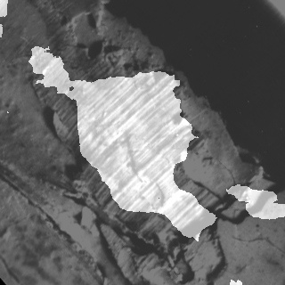
# Quick start: using OpenCV backend {#gapi_anisotropic_start}

Before we start, let's review the original algorithm implementation:

@include cpp/tutorial_code/ImgProc/anisotropic_image_segmentation/anisotropic_image_segmentation.cpp

## Examining calcGST() {#gapi_anisotropic_calcgst}

The function calcGST() is clearly an image processing pipeline:
* It is just a sequence of operations over a number of cv::Mat;
* No logic (conditionals) and loops involved in the code;
* All functions operate on 2D images (like cv::Sobel, cv::multiply,
cv::boxFilter, cv::sqrt, etc).

Considering the above, calcGST() is a great candidate to start
with. In the original code, its prototype is defined like this:

@snippet cpp/tutorial_code/ImgProc/anisotropic_image_segmentation/anisotropic_image_segmentation.cpp calcGST_proto

With G-API, we can define it as follows:

@snippet cpp/tutorial_code/gapi/porting_anisotropic_image_segmentation/porting_anisotropic_image_segmentation_gapi.cpp calcGST_proto

It is important to understand that the new G-API based version of
calcGST() will just produce a compute graph, in contrast to its
original version, which actually calculates the values. This is a
principal difference -- G-API based functions like this are used to
construct graphs, not to process the actual data.

Let's start implementing calcGST() with calculation of \f$J\f$
matrix. This is how the original code looks like:

@snippet cpp/tutorial_code/ImgProc/anisotropic_image_segmentation/anisotropic_image_segmentation.cpp calcJ_header

Here we need to declare output objects for every new operation (see
img as a result for cv::Mat::convertTo, imgDiffX and others as results for
cv::Sobel and cv::multiply).

The G-API analogue is listed below:

@snippet cpp/tutorial_code/gapi/porting_anisotropic_image_segmentation/porting_anisotropic_image_segmentation_gapi.cpp calcGST_header

This snippet demonstrates the following syntactic difference between
G-API and traditional OpenCV:
* All standard G-API functions are by default placed in "cv::gapi"
namespace;
* G-API operations _return_ its results -- there's no need to pass
extra "output" parameters to the functions.

Note -- this code is also using `auto` -- types of intermediate objects
like `img`, `imgDiffX`, and so on are inferred automatically by the
C++ compiler. In this example, the types are determined by G-API
operation return values which all are cv::GMat.

G-API standard kernels are trying to follow OpenCV API conventions
whenever possible -- so cv::gapi::sobel takes the same arguments as
cv::Sobel, cv::gapi::mul follows cv::multiply, and so on (except
having a return value).

The rest of calcGST() function can be implemented the same
way trivially. Below is its full source code:

@snippet cpp/tutorial_code/gapi/porting_anisotropic_image_segmentation/porting_anisotropic_image_segmentation_gapi.cpp calcGST

## Running G-API graph {#gapi_anisotropic_running}

After calcGST() is defined in G-API language, we can construct a graph
based on it and finally run it -- pass input image and obtain
result. Before we do it, let's have a look how original code looked
like:

@snippet cpp/tutorial_code/ImgProc/anisotropic_image_segmentation/anisotropic_image_segmentation.cpp main_extra

G-API-based functions like calcGST() can't be applied to input data
directly, since it is a _construction_ code, not the _processing_ code.
In order to _run_ computations, a special object of class
cv::GComputation needs to be created. This object wraps our G-API code
(which is a composition of G-API data and operations) into a callable
object, similar to C++11
[std::function<>](https://en.cppreference.com/w/cpp/utility/functional/function).

cv::GComputation class has a number of constructors which can be used
to define a graph. Generally, user needs to pass graph boundaries
-- _input_ and _output_ objects, on which a GComputation is
defined. Then G-API analyzes the call flow from _outputs_ to _inputs_
and reconstructs the graph with operations in-between the specified
boundaries. This may sound complex, however in fact the code looks
like this:

@snippet cpp/tutorial_code/gapi/porting_anisotropic_image_segmentation/porting_anisotropic_image_segmentation_gapi.cpp main

Note that this code slightly changes from the original one: forming up
the resulting image is also a part of the pipeline (done with
cv::gapi::addWeighted).

Result of this G-API pipeline bit-exact matches the original one
(given the same input image):

![Segmentation result with G-API](pics/result.jpg)

## G-API initial version: full listing {#gapi_anisotropic_ocv}

Below is the full listing of the initial anisotropic image
segmentation port on G-API:

@snippet cpp/tutorial_code/gapi/porting_anisotropic_image_segmentation/porting_anisotropic_image_segmentation_gapi.cpp full_sample

# Inspecting the initial version {#gapi_anisotropic_inspect}

After we have got the initial working version of our algorithm working
with G-API, we can use it to inspect and learn how G-API works. This
chapter covers two aspects: understanding the graph structure, and
memory profiling.

## Understanding the graph structure {#gapi_anisotropic_inspect_graph}

G-API stands for "Graph API", but did you mention any graphs in the
above example? It was one of the initial design goals -- G-API was
designed with expressions in mind to make adoption and porting process
more straightforward. People _usually_ don't think in terms of
_Nodes_ and _Edges_ when writing ordinary code, and so G-API, while
being a Graph API, doesn't force its users to do that.

However, a graph is still built implicitly when a cv::GComputation
object is defined. It may be useful to inspect how the resulting graph
looks like to check if it is generated correctly and if it really
represents our algorithm. It is also useful to learn the structure of
the graph to see if it has any redundancies.

G-API allows to dump generated graphs to `.dot` files which then
could be visualized with [Graphviz](https://www.graphviz.org/), a
popular open graph visualization software.

<!-- TODO THIS VARIABLE NEEDS TO BE FIXED TO DUMP DIR ASAP! -->

In order to dump our graph to a `.dot` file, set `GRAPH_DUMP_PATH` to a
file name before running the application, e.g.:

    $ GRAPH_DUMP_PATH=segm.dot ./bin/example_tutorial_porting_anisotropic_image_segmentation_gapi

Now this file can be visualized with a `dot` command like this:

    $ dot segm.dot -Tpng -o segm.png

or viewed interactively with `xdot` (please refer to your
distribution/operating system documentation on how to install these
packages).

![Anisotropic image segmentation graph](pics/segm.gif)

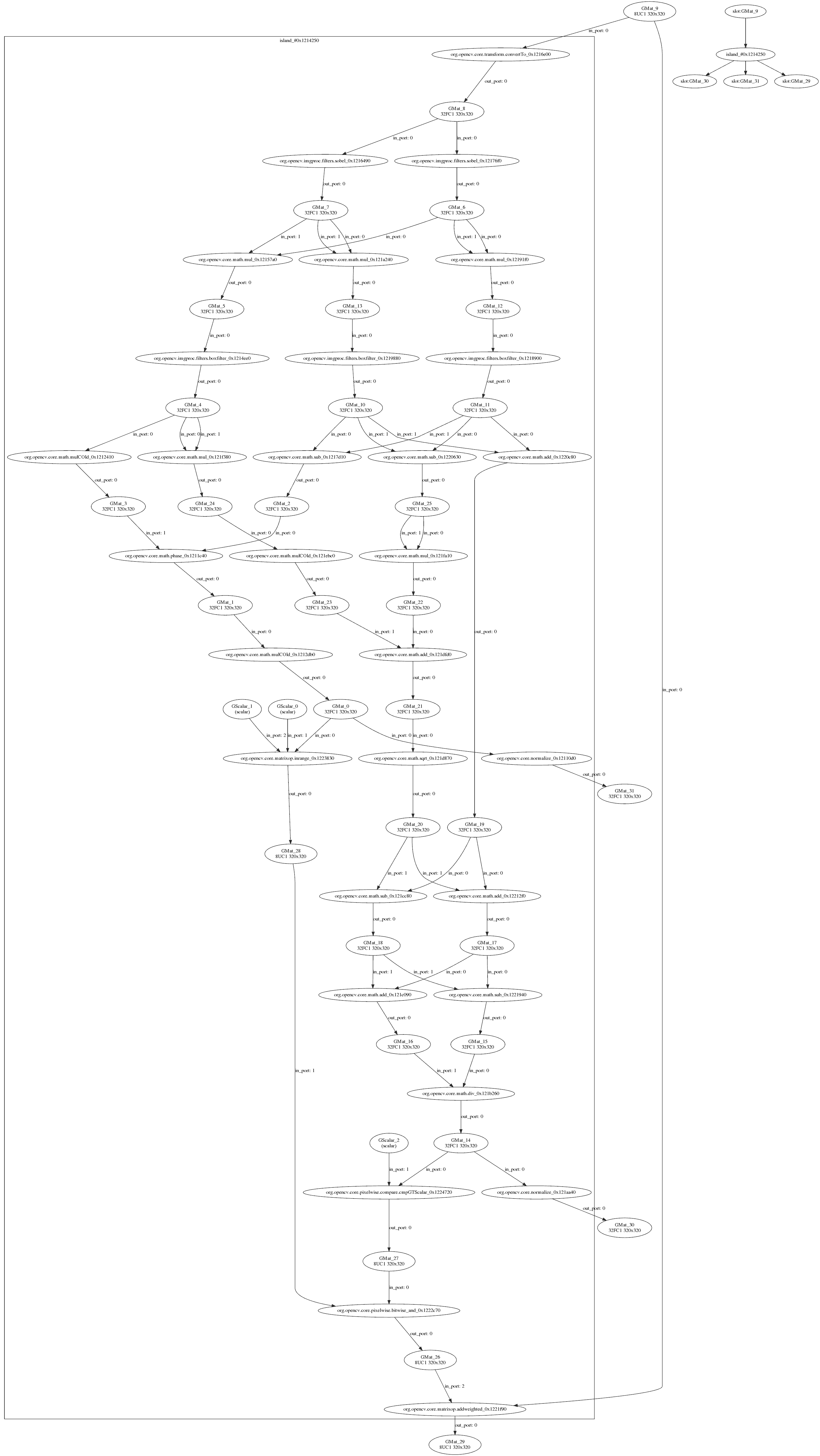
The above diagram demonstrates a number of interesting aspects of
G-API's internal algorithm representation:
1. G-API underlying graph is a bipartite graph: it consists of
   _Operation_ and _Data_ nodes such that a _Data_ node can only be
   connected to an _Operation_ node, _Operation_ node can only be
   connected to a _Data_ node, and nodes of a single kind are never
   connected directly.
2. Graph is directed - every edge in the graph has a direction.
3. Graph "begins" and "ends" with a _Data_ kind of nodes.
4. A _Data_ node can have only a single writer and multiple readers.
5. An _Operation_ node may have multiple inputs, though every input
   must have an unique _port number_ (among inputs).
6. An _Operation_ node may have multiple outputs, and every output
   must have an unique _port number_ (among outputs).

## Measuring memory footprint {#gapi_anisotropic_memory_ocv}

Let's measure and compare memory footprint of the algorithm in its two
versions: G-API-based and OpenCV-based. At the moment, G-API version
is also OpenCV-based since it fallbacks to OpenCV functions inside.

On GNU/Linux, application memory footprint can be profiled with
[Valgrind](http://valgrind.org/). On Debian/Ubuntu systems it can be
installed like this (assuming you have administrator privileges):

    $ sudo apt-get install valgrind massif-visualizer

Once installed, we can collect memory profiles easily for our two
algorithm versions:

    $ valgrind --tool=massif --massif-out-file=ocv.out ./bin/example_tutorial_anisotropic_image_segmentation
    ==6101== Massif, a heap profiler
    ==6101== Copyright (C) 2003-2015, and GNU GPL'd, by Nicholas Nethercote
    ==6101== Using Valgrind-3.11.0 and LibVEX; rerun with -h for copyright info
    ==6101== Command: ./bin/example_tutorial_anisotropic_image_segmentation
    ==6101==
    ==6101==
    $ valgrind --tool=massif --massif-out-file=gapi.out ./bin/example_tutorial_porting_anisotropic_image_segmentation_gapi
    ==6117== Massif, a heap profiler
    ==6117== Copyright (C) 2003-2015, and GNU GPL'd, by Nicholas Nethercote
    ==6117== Using Valgrind-3.11.0 and LibVEX; rerun with -h for copyright info
    ==6117== Command: ./bin/example_tutorial_porting_anisotropic_image_segmentation_gapi
    ==6117==
    ==6117==

Once done, we can inspect the collected profiles with
[Massif Visualizer](https://github.com/KDE/massif-visualizer)
(installed in the above step).

Below is the visualized memory profile of the original OpenCV version
of the algorithm:

![Memory profile: original Anisotropic Image Segmentation sample](pics/massif_export_ocv.png)

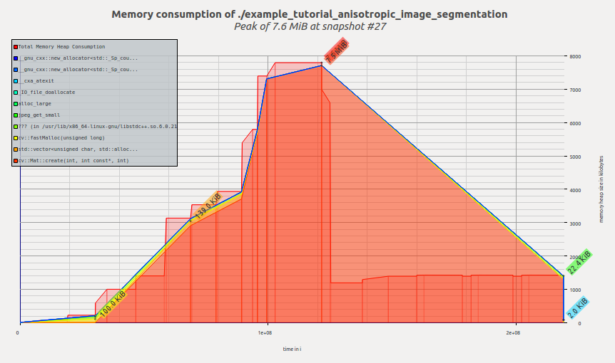
We see that memory is allocated as the application
executes, reaching its peak in the calcGST() function; then the
footprint drops as calcGST() completes its execution and all temporary
buffers are freed. Massif reports us peak memory consumption of 7.6 MiB.

Now let's have a look on the profile of G-API version:

![Memory profile: G-API port of Anisotropic Image Segmentation sample](pics/massif_export_gapi.png)

Once G-API computation is created and its execution starts, G-API
allocates all required memory at once and then the memory profile
remains flat until the termination of the program. Massif reports us
peak memory consumption of 11.4 MiB.

A reader may ask a right question at this point -- is G-API that bad?
What is the reason in using it than?

Hopefully, it is not. The reason why we see here an increased memory
consumption is because the default naive OpenCV-based backend is used to
execute this graph. This backend serves mostly for quick prototyping
and debugging algorithms before offload/further optimization.

This backend doesn't utilize any complex memory management strategies yet
since it is not its point at the moment. In the following chapter,
we'll learn about Fluid backend and see how the same G-API code can
run in a completely different model (and the footprint shrunk to a
number of kilobytes).

# Backends and kernels {#gapi_anisotropic_backends}

This chapter covers how a G-API computation can be executed in a
special way -- e.g. offloaded to another device, or scheduled with a
special intelligence. G-API is designed to make its graphs portable --
it means that once a graph is defined in G-API terms, no changes
should be required in it if we want to run it on CPU or on GPU or on
both devices at once. [G-API High-level overview](@ref gapi_hld) and
[G-API Kernel API](@ref gapi_kernel_api) shed more light on technical
details which make it possible. In this chapter, we will utilize G-API
Fluid backend to make our graph cache-efficient on CPU.

G-API defines _backend_ as the lower-level entity which knows how to
run kernels. Backends may have (and, in fact, do have) different
_Kernel APIs_ which are used to program and integrate kernels for that
backends. In this context, _kernel_ is an implementation of an
_operation_, which is defined on the top API level (see
G_TYPED_KERNEL() macro).

Backend is a thing which is aware of device & platform specifics, and
which executes its kernels with keeping that specifics in mind. For
example, there may be [Halide](http://halide-lang.org/) backend which
allows to write (implement) G-API operations in Halide language and
then generate functional Halide code for portions of G-API graph which
map well there.

## Running a graph with a Fluid backend {#gapi_anisotropic_fluid}

OpenCV 4.0 is bundled with two G-API backends -- the default "OpenCV"
which we just used, and a special "Fluid" backend.

Fluid backend reorganizes the execution to save memory and to achieve
near-perfect cache locality, implementing so-called "streaming" model
of execution.

In order to start using Fluid kernels, we need first to include
appropriate header files (which are not included by default):

@snippet cpp/tutorial_code/gapi/porting_anisotropic_image_segmentation/porting_anisotropic_image_segmentation_gapi_fluid.cpp fluid_includes

Once these headers are included, we can form up a new _kernel package_
and specify it to G-API:

@snippet cpp/tutorial_code/gapi/porting_anisotropic_image_segmentation/porting_anisotropic_image_segmentation_gapi_fluid.cpp kernel_pkg

In G-API, kernels (or operation implementations) are objects. Kernels are
organized into collections, or _kernel packages_, represented by class
cv::GKernelPackage. The main purpose of a kernel package is to
capture which kernels we would like to use in our graph, and pass it
as a _graph compilation option_:

@snippet cpp/tutorial_code/gapi/porting_anisotropic_image_segmentation/porting_anisotropic_image_segmentation_gapi_fluid.cpp kernel_pkg_use

Traditional OpenCV is logically divided into modules, with every
module providing a set of functions. In G-API, there are also
"modules" which are represented as kernel packages provided by a
particular backend. In this example, we pass Fluid kernel packages to
G-API to utilize appropriate Fluid functions in our graph.

Kernel packages are combinable -- in the above example, we take "Core"
and "ImgProc" Fluid kernel packages and combine it into a single
one. See documentation reference on cv::gapi::combine.

If no kernel packages are specified in options, G-API is using
_default_ package which consists of default OpenCV implementations and
thus G-API graphs are executed via OpenCV functions by default. OpenCV
backend provides broader functional coverage than any other
backend. If a kernel package is specified, like in this example, then
it is being combined with the _default_.
It means that user-specified implementations will replace default implementations in case of
conflict.

<!-- FIXME Document this process better as a part of regular -->
<!-- documentation, not a tutorial kind of thing -->

## Troubleshooting and customization {#gapi_anisotropic_trouble}

After the above modifications, (in OpenCV 4.0) the app should crash
with a message like this:

```
$ ./bin/example_tutorial_porting_anisotropic_image_segmentation_gapi_fluid
terminate called after throwing an instance of 'std::logic_error'
  what():  .../modules/gapi/src/backends/fluid/gfluidimgproc.cpp:436: Assertion kernelSize.width == 3 && kernelSize.height == 3 in function run failed

Aborted (core dumped)
```

Fluid backend has a number of limitations in OpenCV 4.0 (see this
[wiki page](https://github.com/opencv/opencv/wiki/Graph-API) for a
more up-to-date status). In particular, the Box filter used in this
sample supports only static 3x3 kernel size.

We can overcome this problem easily by avoiding G-API using Fluid
version of Box filter kernel in this sample. It can be done by
removing the appropriate kernel from the kernel package we've just
created:

@snippet cpp/tutorial_code/gapi/porting_anisotropic_image_segmentation/porting_anisotropic_image_segmentation_gapi_fluid.cpp kernel_hotfix

Now this kernel package doesn't have _any_ implementation of Box
filter kernel interface (specified as a template parameter). As
described above, G-API will fall-back to OpenCV to run this kernel
now. The resulting code with this change now looks like:

@snippet cpp/tutorial_code/gapi/porting_anisotropic_image_segmentation/porting_anisotropic_image_segmentation_gapi_fluid.cpp kernel_pkg_proper

Let's examine the memory profile for this sample after we switched to
Fluid backend. Now it looks like this:

![Memory profile: G-API/Fluid port of Anisotropic Image Segmentation sample](pics/massif_export_gapi_fluid.png)

Now the tool reports 4.7MiB -- and we just changed a few lines in our
code, without modifying the graph itself! It is a ~2.4X improvement of
the previous G-API result, and ~1.6X improvement of the original OpenCV
version.

Let's also examine how the internal representation of the graph now
looks like. Dumping the graph into `.dot` would result into a
visualization like this:

![Anisotropic image segmentation graph with OpenCV & Fluid kernels](pics/segm_fluid.gif)

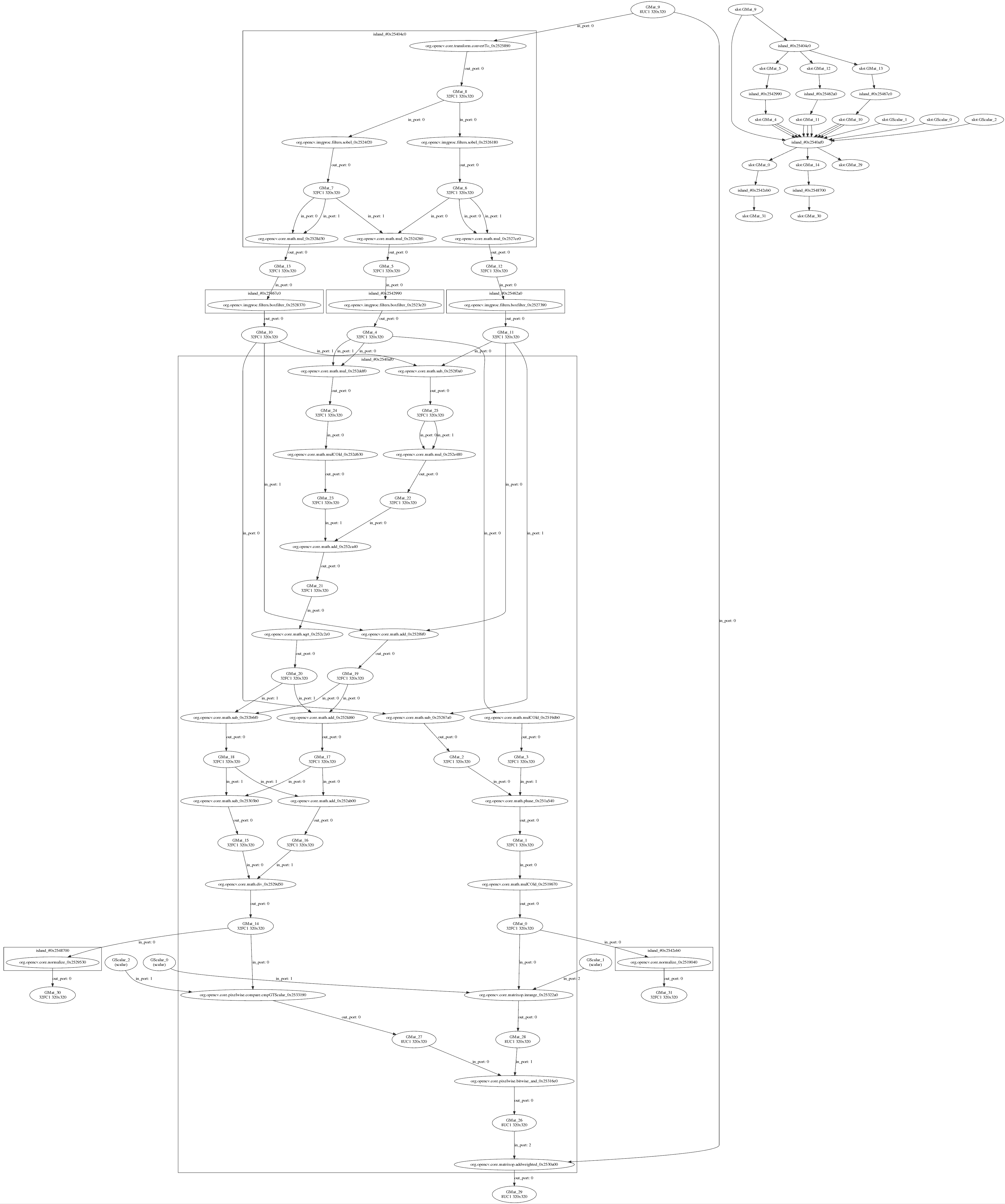
This graph doesn't differ structurally from its previous version (in
terms of operations and data objects), though a changed layout (on the
left side of the dump) is easily noticeable.

The visualization reflects how G-API deals with mixed graphs, also
called _heterogeneous_ graphs. The majority of operations in this
graph are implemented with Fluid backend, but Box filters are executed
by the OpenCV backend. One can easily see that the graph is partitioned
(with rectangles). G-API groups connected operations based on their
affinity, forming _subgraphs_ (or _islands_ in G-API terminology), and
our top-level graph becomes a composition of multiple smaller
subgraphs. Every backend determines how its subgraph (island) is
executed, so Fluid backend optimizes out memory where possible, and
six intermediate buffers accessed by OpenCV Box filters are allocated
fully and can't be optimized out.

<!-- TODO: add a chapter on custom kernels -->
<!-- TODO: make a full-fluid pipeline -->
<!-- TODO: talk about parallelism when it is available -->

# Conclusion {#gapi_tutor_conclusion}

This tutorial demonstrates what G-API is and what its key design
concepts are, how an algorithm can be ported to G-API, and
how to utilize graph model benefits after that.

In OpenCV 4.0, G-API is still in its inception stage -- it is more a
foundation for all future work, though ready for use even now.

Further, this tutorial will be extended with new chapters on custom
kernels programming, parallelism, and more.