1
2
3
4
5
6
7
8
9
10
11
12
13
14
15
16
17
18
19
20
21
22
23
24
25
26
27
28
29
30
31
32
33
34
35
36
37
38
39
40
41
42
43
44
45
46
47
48
49
50
51
52
53
54
55
56
57
58
59
60
61
62
63
64
65
66
67
68
69
70
71
72
73
74
75
76
77
78
79
80
81
82
83
84
85
86
87
88
89
90
91
92
93
94
95
96
97
98
99
100
101
102
103
104
105
106
107
108
109
110
111
112
113
114
115
116
117
118
119
120
121
122
123
124
125
126
127
128
129
130
131
132
133
134
135
136
137
138
139
140
141
142
143
144
145
146
147
148
149
150
151
152
153
154
155
156
157
158
159
160
161
162
163
164
165
166
167
168
169
170
171
172
173
174
175
176
177
178
179
180
181
182
183
184
185
186
187
188
189
190
191
192
193
194
195
196
|
Histogram Comparison {#tutorial_histogram_comparison}
====================
@tableofcontents
@prev_tutorial{tutorial_histogram_calculation}
@next_tutorial{tutorial_back_projection}
| | |
| -: | :- |
| Original author | Ana Huamán |
| Compatibility | OpenCV >= 3.0 |
Goal
----
In this tutorial you will learn how to:
- Use the function @ref cv::compareHist to get a numerical parameter that express how well two
histograms match with each other.
- Use different metrics to compare histograms
Theory
------
- To compare two histograms ( \f$H_{1}\f$ and \f$H_{2}\f$ ), first we have to choose a *metric*
(\f$d(H_{1}, H_{2})\f$) to express how well both histograms match.
- OpenCV implements the function @ref cv::compareHist to perform a comparison. It also offers 4
different metrics to compute the matching:
-# **Correlation ( CV_COMP_CORREL )**
\f[d(H_1,H_2) = \frac{\sum_I (H_1(I) - \bar{H_1}) (H_2(I) - \bar{H_2})}{\sqrt{\sum_I(H_1(I) - \bar{H_1})^2 \sum_I(H_2(I) - \bar{H_2})^2}}\f]
where
\f[\bar{H_k} = \frac{1}{N} \sum _J H_k(J)\f]
and \f$N\f$ is the total number of histogram bins.
-# **Chi-Square ( CV_COMP_CHISQR )**
\f[d(H_1,H_2) = \sum _I \frac{\left(H_1(I)-H_2(I)\right)^2}{H_1(I)}\f]
-# **Intersection ( method=CV_COMP_INTERSECT )**
\f[d(H_1,H_2) = \sum _I \min (H_1(I), H_2(I))\f]
-# **Bhattacharyya distance ( CV_COMP_BHATTACHARYYA )**
\f[d(H_1,H_2) = \sqrt{1 - \frac{1}{\sqrt{\bar{H_1} \bar{H_2} N^2}} \sum_I \sqrt{H_1(I) \cdot H_2(I)}}\f]
Code
----
- **What does this program do?**
- Loads a *base image* and 2 *test images* to be compared with it.
- Generate 1 image that is the lower half of the *base image*
- Convert the images to HSV format
- Calculate the H-S histogram for all the images and normalize them in order to compare them.
- Compare the histogram of the *base image* with respect to the 2 test histograms, the
histogram of the lower half base image and with the same base image histogram.
- Display the numerical matching parameters obtained.
@add_toggle_cpp
- **Downloadable code**: Click
[here](https://github.com/opencv/opencv/tree/4.x/samples/cpp/tutorial_code/Histograms_Matching/compareHist_Demo.cpp)
- **Code at glance:**
@include samples/cpp/tutorial_code/Histograms_Matching/compareHist_Demo.cpp
@end_toggle
@add_toggle_java
- **Downloadable code**: Click
[here](https://github.com/opencv/opencv/tree/4.x/samples/java/tutorial_code/Histograms_Matching/histogram_comparison/CompareHistDemo.java)
- **Code at glance:**
@include samples/java/tutorial_code/Histograms_Matching/histogram_comparison/CompareHistDemo.java
@end_toggle
@add_toggle_python
- **Downloadable code**: Click
[here](https://github.com/opencv/opencv/tree/4.x/samples/python/tutorial_code/Histograms_Matching/histogram_comparison/compareHist_Demo.py)
- **Code at glance:**
@include samples/python/tutorial_code/Histograms_Matching/histogram_comparison/compareHist_Demo.py
@end_toggle
Explanation
-----------
- Load the base image (src_base) and the other two test images:
@add_toggle_cpp
@snippet samples/cpp/tutorial_code/Histograms_Matching/compareHist_Demo.cpp Load three images with different environment settings
@end_toggle
@add_toggle_java
@snippet samples/java/tutorial_code/Histograms_Matching/histogram_comparison/CompareHistDemo.java Load three images with different environment settings
@end_toggle
@add_toggle_python
@snippet samples/python/tutorial_code/Histograms_Matching/histogram_comparison/compareHist_Demo.py Load three images with different environment settings
@end_toggle
- Convert them to HSV format:
@add_toggle_cpp
@snippet samples/cpp/tutorial_code/Histograms_Matching/compareHist_Demo.cpp Convert to HSV
@end_toggle
@add_toggle_java
@snippet samples/java/tutorial_code/Histograms_Matching/histogram_comparison/CompareHistDemo.java Convert to HSV
@end_toggle
@add_toggle_python
@snippet samples/python/tutorial_code/Histograms_Matching/histogram_comparison/compareHist_Demo.py Convert to HSV
@end_toggle
- Also, create an image of half the base image (in HSV format):
@add_toggle_cpp
@snippet samples/cpp/tutorial_code/Histograms_Matching/compareHist_Demo.cpp Convert to HSV half
@end_toggle
@add_toggle_java
@snippet samples/java/tutorial_code/Histograms_Matching/histogram_comparison/CompareHistDemo.java Convert to HSV half
@end_toggle
@add_toggle_python
@snippet samples/python/tutorial_code/Histograms_Matching/histogram_comparison/compareHist_Demo.py Convert to HSV half
@end_toggle
- Initialize the arguments to calculate the histograms (bins, ranges and channels H and S ).
@add_toggle_cpp
@snippet samples/cpp/tutorial_code/Histograms_Matching/compareHist_Demo.cpp Using 50 bins for hue and 60 for saturation
@end_toggle
@add_toggle_java
@snippet samples/java/tutorial_code/Histograms_Matching/histogram_comparison/CompareHistDemo.java Using 50 bins for hue and 60 for saturation
@end_toggle
@add_toggle_python
@snippet samples/python/tutorial_code/Histograms_Matching/histogram_comparison/compareHist_Demo.py Using 50 bins for hue and 60 for saturation
@end_toggle
- Calculate the Histograms for the base image, the 2 test images and the half-down base image:
@add_toggle_cpp
@snippet samples/cpp/tutorial_code/Histograms_Matching/compareHist_Demo.cpp Calculate the histograms for the HSV images
@end_toggle
@add_toggle_java
@snippet samples/java/tutorial_code/Histograms_Matching/histogram_comparison/CompareHistDemo.java Calculate the histograms for the HSV images
@end_toggle
@add_toggle_python
@snippet samples/python/tutorial_code/Histograms_Matching/histogram_comparison/compareHist_Demo.py Calculate the histograms for the HSV images
@end_toggle
- Apply sequentially the 4 comparison methods between the histogram of the base image (hist_base)
and the other histograms:
@add_toggle_cpp
@snippet samples/cpp/tutorial_code/Histograms_Matching/compareHist_Demo.cpp Apply the histogram comparison methods
@end_toggle
@add_toggle_java
@snippet samples/java/tutorial_code/Histograms_Matching/histogram_comparison/CompareHistDemo.java Apply the histogram comparison methods
@end_toggle
@add_toggle_python
@snippet samples/python/tutorial_code/Histograms_Matching/histogram_comparison/compareHist_Demo.py Apply the histogram comparison methods
@end_toggle
Results
-------
-# We use as input the following images:


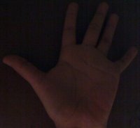
where the first one is the base (to be compared to the others), the other 2 are the test images.
We will also compare the first image with respect to itself and with respect of half the base
image.
-# We should expect a perfect match when we compare the base image histogram with itself. Also,
compared with the histogram of half the base image, it should present a high match since both
are from the same source. For the other two test images, we can observe that they have very
different lighting conditions, so the matching should not be very good:
-# Here the numeric results we got with OpenCV 3.4.1:
*Method* | Base - Base | Base - Half | Base - Test 1 | Base - Test 2
----------------- | ------------ | ------------ | -------------- | ---------------
*Correlation* | 1.000000 | 0.880438 | 0.20457 | 0.0664547
*Chi-square* | 0.000000 | 4.6834 | 2697.98 | 4763.8
*Intersection* | 18.8947 | 13.022 | 5.44085 | 2.58173
*Bhattacharyya* | 0.000000 | 0.237887 | 0.679826 | 0.874173
For the *Correlation* and *Intersection* methods, the higher the metric, the more accurate the
match. As we can see, the match *base-base* is the highest of all as expected. Also we can observe
that the match *base-half* is the second best match (as we predicted). For the other two metrics,
the less the result, the better the match. We can observe that the matches between the test 1 and
test 2 with respect to the base are worse, which again, was expected.
|
