1
2
3
4
5
6
7
8
9
10
11
12
13
14
15
16
17
18
19
20
21
22
23
24
25
26
27
28
29
30
31
32
33
34
35
36
37
38
39
40
41
42
43
44
45
46
47
48
49
50
51
52
53
54
55
56
57
58
59
60
61
62
63
64
65
66
67
68
69
70
71
72
73
74
75
76
77
78
79
80
81
82
83
84
85
86
87
88
89
90
91
92
93
94
95
96
97
98
99
100
101
102
103
104
105
106
107
108
109
110
111
112
113
114
115
116
117
118
119
120
121
122
123
124
125
126
127
128
129
130
131
132
133
134
135
136
137
138
139
140
141
142
143
144
145
146
147
148
149
150
151
152
153
154
155
156
157
158
159
160
161
162
163
164
165
166
167
168
169
170
171
172
173
174
175
176
177
178
179
180
181
182
183
184
185
186
187
188
189
190
191
192
193
194
195
196
197
198
199
200
201
202
203
204
205
206
207
208
209
210
211
212
213
214
215
216
217
218
219
220
221
222
223
224
225
226
227
228
229
230
231
232
233
234
235
236
237
238
239
240
241
242
243
244
245
246
247
248
249
250
251
|
# Structured Pruning
## Intro / Motivation
**Pruning** is the technique of removing parameters from a model to reduce the computational cost. The goal of pruning is to improve the performance of the model while maintaining it's accuracy.
### Unstructured vs. Structured Pruning
One way to do this is to consider each parameter individually. This gives us the greatest granularity when pruning and is called **unstructured pruning**.
For example, consider a simple linear regression model that is parametrized by a weight tensor W.
```
W = [[1 2 3]
[4 5 6]
[7 1 9]]
```
We can prune the lowest absolute value elements in W in order to preserve as much information as possible.
Below we've removed three parameters from W.
```
W_pruned = [[0 0 3]
[4 5 6]
[7 0 9]]
```
Unfortunately, zeroing out parameters does not offer a speed-up to the model out of the box. We need custom sparse kernels that are designed to take advantage of sparsity to speed up computation. For more information about unstructured pruning check out our tutorials [here]().
However, if we zero out a row of parameters at a time instead of a single parameter, we can speed up computation by resizing the weight matrix. This is called **structured pruning** and is what this folder implements.
```
W_pruned = [[0 0 0] = [[4, 5, 6],
[4 5 6] [7, 1, 9]]
[7 1 9]]
```
### Weight Resizing
However, since the pruned weight tensor has a different shape than the original weight tensor, subsequent operations will cause an error due to this shape mismatch. We need to remove both the weights of the original weight tensor and the columns of subsequent tensors that correspond to the pruned rows.
You can see an example of this below for a model containing two linear layers, one parametrized by W and another by U
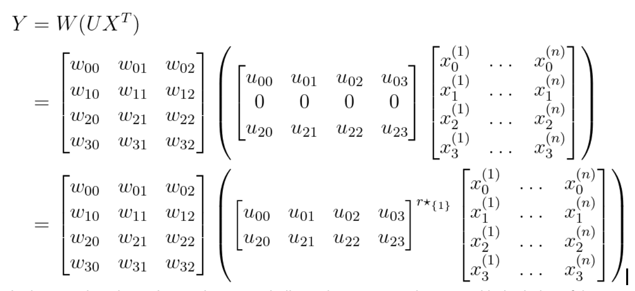
By removing a row from U and a column from W, we can avoid a shape mismatch.

One benefit of **structured pruning** is that it uses the same dense kernels that the original model uses, and does not rely on custom sparse kernel like **unstructured pruning**.
However, structured pruning degrades accuracy more than unstructured pruning because of the lack of granularity, so it is not always the right choice.
Generally the structured pruning process looks something like this:
1. Define what layers in the model you want to structured prune.
2. Evaluate the importance of each row in each layer in the model.
3. Remove rows by resizing the weight matrices of each layer
4. Stop if target sparsity level is met.
The accuracy degradation of pruning can be quite large initially. Once we are satisfied with our pruned tensor, we usually retrain the model after pruning in order to restore some of this accuracy loss.
## Quickstart Guide
**Your model must be FX symbolically traceable**.
You can test this with the following bit of code:
```python
from torch.fx import symbolic_trace
model = MyModel()
symbolic_trace(model)
```
Using `torch.fx` we can get a compute graph of our model. Each operation (add, multiply, ReLU) is a node in the graph, and the order of operations is defined by the edges of the graph.
Structured pruning works by traversing this graph and looking for specific **patterns**, which are just a specific sequence of operations.
Each pattern is tied to a pruning function, which is responsible for structured pruning the graph nodes that match the pattern.
The above [example](#weight-resizing) of two linear layers would match against a `(nn.Linear, nn.Linear)` pattern. This is how we identify the rows to remove and the columns of the subsequent layer.
Structured pruning also works on other patterns other than two adjacent Linear layers,
- linear -> linear
- linear -> activation -> linear
- conv2d -> conv2d
- conv2d -> activation -> conv2d
- conv2d -> activation -> pool -> conv2d
- conv2d -> pool -> activation -> conv2d
- conv2d -> adaptive pool -> flatten -> linear
A complete set of the patterns we support can be found [here](https://github.com/pytorch/pytorch/blob/master/torch/ao/pruning/_experimental/pruner/base_structured_sparsifier.py#L85).
If you are looking to prune a currently unsupported pattern, you can do this by modifying the pattern dict that we provide to the pruner, see [here](#writing-custom-patterns-and-pruning-functions-for-structured-pruning). Feel free to open a PR to add in new patterns.
Here is an example script that will prune away 50% of the rows for all the linear layers in the model, based on the saliency of each row.
```python
from torch.ao.pruning._experimental.pruner import SaliencyPruner
# Define model
class Model(nn.Module):
def __init__(self) -> None:
super().__init__()
self.seq = nn.Sequential(
nn.Linear(700, 500, bias=True),
nn.ReLU(),
nn.Linear(500, 800, bias=False),
nn.ReLU(),
nn.Linear(800, 600, bias=True),
nn.ReLU(),
)
self.linear = nn.Linear(600, 4, bias=False)
def forward(self, x):
x = self.seq(x)
x = self.linear(x)
return x
# Define pruning_config, which specifies which tensors you wish to prune.
# The SaliencyPruner also needs a sparsity_level parameter to specify what % of rows to prune.
pruning_config = [
{"tensor_fqn": "seq.0.weight", "sparsity_level": 0.5},
{"tensor_fqn": "seq.2.weight", "sparsity_level": 0.5},
{"tensor_fqn": "seq.4.weight", "sparsity_level": 0.5},
{"tensor_fqn": "linear.weight", "sparsity_level": 0.5},
]
original = Model()
# define defaults
# for structured pruning, we also prune biases by default.
defaults = {"prune_bias": True}
# any configs passed in here are defaults that are propagated
# Your selection criteria is decided by which pruner you use
pruner = SaliencyPruner(defaults, patterns=patterns)
# Next we call `prepare`, which will attach `FakeStructuredSparsity` parameterizations
# to the tensors specified in the config. These parameterizations will zero out
# the appropriate weights in order to make the model behave as if it has been pruned.
pruner.prepare(original, sparse_config)
# take one pruning step. This will update the masks
pruner.enable_mask_update = True
pruner.step()
# pruner.prune() will find patterns and apply that patterns pruning function to it's matching nodes.
# The output of pruner.prune() is a model with resized weights and the masks / parametrizations removed.
pruned_model = pruner.prune()
```
Afterwards, by printing the name and size of each parameter in our model, we can see that it has been pruned.
```
# original model
Parameter name | Shape | # of elements
--------------------|-----------------|---------------
seq.0.weight | 500, 700 | 350000
seq.0.bias | 500 | 500
seq.2.weight | 800, 500 | 400000
seq.4.weight | 600, 800 | 480000
seq.4.bias | 600 | 600
linear.weight | 4, 600 | 2400
=== Total Number of Parameters: 1233500 ===
```
```
# pruned model
Parameter name | Shape | # of elements
--------------------|-----------------|---------------
seq.0.weight | 250, 700 | 175000
seq.0.bias | 250 | 250
seq.2.weight | 400, 250 | 100000
seq.4.weight | 300, 400 | 120000
seq.4.bias | 300 | 300
linear.weight | 2, 300 | 600
=== Total Number of Parameters: 396150 ===
```
Although we pruned 50% of the rows, the total number of parameters is 25% of the original model.
Since we remove both the rows of a weight tensor and the columns of the subsequent tensor. The total number of parameters is roughly (1-0.5)* (1-0.5) = 0.25 of the original number of parameters.
## Advanced Tutorial
### Pruning Config
To specify the layers to prune we just need the fully qualified name (FQN) of the tensor you are looking to prune in the module.
You can get the FQN of a tensor by printing out `model.named_parameters()`.
To prune multiple layers, we just append entries to the pruning config.
**tensor_fqn** is the only required key in the pruning config. You can pass additional information in the config, for example the sparsity level you want to prune to by adding a key to the config. You can then access this additional information when you update the masks.
### Implementing a Pruner
If you want to prune weights using a different pruning criteria than saliency, you'll need to implement your own pruner.
To do this, we need to extend a `BaseStructuredSparsifier` with a custom `update_mask` function.
This `update_mask` function contains the user logic for picking what weights to prune.
One common pruning criteria is to use the **saliency** of a row, which is defined as the sum of all the L1 norms of the weights in the row.
The idea is to remove the weights that are small, since they wouldn't contribute much to the final prediction.
Below we can see an implemented Saliency Pruner
```python
class SaliencyPruner(BaseStructuredSparsifier):
"""
Prune filters based on the saliency
The saliency for a filter is given by the sum of the L1 norms of all of its weights
"""
def update_mask(self, module, tensor_name, **kwargs):
# tensor_name will give you the FQN, all other keys in pruning config are present in kwargs
weights = getattr(module, tensor_name)
mask = getattr(module.parametrizations, tensor_name)[0].mask
# use negative weights so we can use topk (we prune out the smallest)
saliency = -weights.norm(dim=tuple(range(1, weights.dim())), p=1)
num_to_pick = int(len(mask) * kwargs["sparsity_level"])
prune = saliency.topk(num_to_pick).indices
# Set the mask to be false for the rows we want to prune
mask.data[prune] = False
```
### Writing Custom Patterns and Pruning Functions for Structured Pruning
If you're working with linear/conv2d layers, it's very probable that you just need to add an entry to the pattern dict mapping your pattern to an existing prune_function.
This is because there are many modules, for example **pooling** that behave the same way and do not need to be modified by the pruning code.
```python
from torch.ao.pruning._experimental.pruner.prune_functions import prune_conv2d_activation_conv2d
def prune_conv2d_pool_activation_conv2d(
c1: nn.Conv2d,
pool: nn.Module,
activation: Optional[Callable[[Tensor], Tensor]],
c2: nn.Conv2d,
) -> None:
prune_conv2d_activation_conv2d(c1, activation, c2)
# note how the pattern defined in the key will be passed to the pruning function as args
my_patterns = {(nn.Conv2d, nn.MaxPool2d, nn.ReLU, nn.Conv2d): prune_conv2d_activation_conv2d}
pruning_patterns = _get_default_structured_pruning_patterns()
pruning_patterns.update(my_patterns)
pruner = SaliencyPruner({}, patterns=pruning_patterns)
```
However, there are also modules like batch norm, which will not work properly without being pruned as well. In this instance, you would need to write a custom pruning function in order to handle that logic properly.
You can see the implemented pruning functions [here](https://github.com/pytorch/pytorch/blob/master/torch/ao/pruning/_experimental/pruner/prune_functions.py) for examples. Please feel free to open a PR so we get a complete set of the patterns and pruning functions.
|
