1
2
3
4
5
6
7
8
9
10
11
12
13
14
15
16
17
18
19
20
21
22
23
24
25
26
27
28
29
30
31
32
33
34
35
36
37
38
39
40
41
42
43
44
45
46
47
48
49
50
51
52
53
54
55
56
57
58
59
60
61
62
63
64
65
66
67
68
69
70
71
72
73
74
75
76
77
78
79
80
81
82
83
84
85
86
87
88
89
90
91
92
93
94
95
96
97
98
99
100
101
102
103
104
105
106
107
108
109
110
111
112
113
114
115
116
117
118
119
120
121
122
123
124
125
126
127
128
129
130
131
132
133
134
135
136
137
138
139
140
141
142
143
144
145
146
147
148
149
150
151
152
153
154
155
156
157
158
159
160
161
162
163
164
165
166
167
168
169
170
171
172
173
174
175
176
177
178
179
180
181
182
183
184
185
186
187
188
189
190
191
192
193
194
195
196
197
198
199
200
201
202
203
204
205
206
207
208
209
210
211
212
213
214
215
216
217
218
219
220
221
222
223
224
225
226
227
228
229
230
231
232
233
234
235
236
237
238
239
240
241
242
243
244
245
246
247
248
249
250
251
252
253
254
255
256
257
258
259
260
261
262
263
264
265
266
267
268
269
270
271
272
273
274
275
276
277
278
279
280
281
282
283
284
285
286
287
288
289
290
291
292
293
294
295
296
297
298
299
300
301
302
303
304
305
306
307
308
309
310
311
312
313
314
315
316
317
318
319
320
321
322
323
324
325
326
327
328
329
330
331
332
333
334
335
336
337
338
339
340
341
342
343
344
345
346
347
348
349
350
351
352
353
354
355
356
357
358
359
360
361
362
363
364
365
366
367
368
369
370
371
372
373
374
375
376
377
378
379
380
381
382
383
384
385
386
387
388
389
390
391
392
393
394
395
396
397
398
399
400
401
402
403
404
405
406
407
408
409
410
411
412
413
414
415
416
417
418
419
420
421
422
423
424
425
426
427
428
429
430
431
432
433
434
435
436
437
438
439
440
441
|
---
title: "Model Specification for Confirmatory Factor Analysis"
date: "`r Sys.Date()`"
output:
html_document:
df_print: paged
toc: true
rmarkdown::html_vignette: default
pdf_document: default
vignette: |
%\VignetteEngine{knitr::knitr}
%\VignetteIndexEntry{Model Specification for Confirmatory Factor Analysis}
%\usepackage[UTF-8]{inputenc}
---
```{r, include = FALSE}
is_CRAN <- !identical(Sys.getenv("NOT_CRAN"), "true")
if (!is_CRAN) {
options(mc.cores = parallel::detectCores())
} else {
knitr::opts_chunk$set(eval = FALSE)
knitr::knit_hooks$set(evaluate.inline = function(x, envir) x)
}
```
This vignette will demonstrate latent variable modeling and confirmatory analysis via the common factor model. Factor analysis is a rudimentary application of OpenMx, and hopefully will serve as an easily understandable introduction to the data structures and workflow patterns necessary to define and fit a model using OpenMx.
OpenMX handles model definition through the `MxModel` class, instantiated via the `mxModel()` function. Model definition requires input data for analysis and the model specification itself. Input data can be either in the form of a set of variable observations or by having a covariance matrix and associated variable means. The model specification can either be produced via specifying a path diagram or, for advanced users, the matrices to define the desired RAM or LISREL model.
We’ll walk through the construction of a single and multiple factor model first through specifying the path diagram, and then an alternate form of model specification manually defining the matrices in a RAM-type model. Additionally, we will demonstrate how to specify data for analysis using either raw data or a covariance matrix of manifest variables. Scripts for [a variety of implementations are located within the `/demo/` directory of the OpenMx GitHub repository](https://github.com/OpenMx/OpenMx/tree/master/demo) and are named in accordance with their specific implementation (eg. "OneFactorModel_PathRaw.R", "TwoFactorModel_MatrixCov.R", etc.)
## Common Factor Model
The common factor model supposes that observed variables measure or indicate the same latent variable. While there are a number of exploratory approaches that do not assume the number of latent factor(s), this example uses a confirmatory approach that assumes a single factor. A path diagram verions of the common factor model for a set of variables $x_{1}-x_{6}$ are given below.
\begin{eqnarray*} x_{ij} = \mu_{j} + \lambda_{j} * \eta_{i} + \epsilon_{ij} \end{eqnarray*}
<center>

</center>
### Multiple Factor Model
The common factor model can be extended to include multiple latent variables. The model for any person and path diagram of the common factor model for a set of variables $x_{1}-x_{3}$ and $y_{1}-y_{3}$ are given below.
\begin{eqnarray*} x_{ij} = \mu_{j} + \lambda_{j} * \eta_{1i} + \epsilon_{ij}\\ y_{ij} = \mu_{j} + \lambda_{j} * \eta_{2i} + \epsilon_{ij} \end{eqnarray*}
<center>
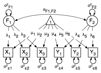
</center>
While 19 parameters are displayed in the equation and path diagram above (six manifest variances, six manifest means, six factor loadings and one factor variance), we must constrain either the factor variance or one factor loading to a constant to identify the model and scale the latent variable. As such, this model contains 18 parameters. The means and covariance matrix for six observed variables contain 27 degrees of freedom, and thus our model contains 9 degrees of freedom.
## Input Data
Our first step to running this model is to include the data to be analyzed. The `MxData` class instantiated through `mxData()` is used for representing data within the `MxModel`.
As mentioned, a raw set of observations on variables can be provided as data. The data for this example is available from the `myFADataRaw` dataset, which contains 500 observations on nine observed variables. In accordance with the path diagram above, we specify the first six variables for analysis in the model.
```{r}
library(OpenMx)
data(myFADataRaw)
dataRawOneFactor <- mxData( observed=myFADataRaw[,c("x1","x2","x3","x4","x5","x6")], type="raw" )
```
Alternatively, our data could be specificed via a covariance matrix with variable means and number of observations. A type argument of `"cov"` is specified in the below example with a covariance matrix (other inputs being the same).
```{r}
myFADataCov<-matrix(
c(0.997, 0.642, 0.611, 0.672, 0.637, 0.677,
0.642, 1.025, 0.608, 0.668, 0.643, 0.676,
0.611, 0.608, 0.984, 0.633, 0.657, 0.626,
0.672, 0.668, 0.633, 1.003, 0.676, 0.665,
0.637, 0.643, 0.657, 0.676, 1.028, 0.654,
0.677, 0.676, 0.626, 0.665, 0.654, 1.020),
nrow=6,
dimnames=list(
c("x1","x2","x3","x4","x5","x6"),
c("x1","x2","x3","x4","x5","x6"))
)
myFADataMeans <- c(2.988, 3.011, 2.986, 3.053, 3.016, 3.010)
names(myFADataMeans) <- c("x1","x2","x3","x4","x5","x6")
dataCovOneFactor <- mxData( observed=myFADataCov, type="cov", numObs=500,
mean=myFADataMeans )
```
### Input Data, Multiple Factors
The only difference in setting up data for multiple factor analysis is to label the manifest variables appropriately. The below code reads in the first six variables from the `myFADataRaw` dataset once again, but this time the labels for $y_n$ observed variables for the second factor, $F_2$ are changed to match the two factor path diagram above. Variable naming is arbitrary and does not affect the model structure.
```{r}
dataRawTwoFactor <- mxData( observed=myFADataRaw[,c("x1","x2","x3","y1","y2","y3")], type="raw" )
```
Setting up a covariance data input for multiple factors involves similar changes from the single factor case. The below code block sets up a covariance matrix of 9 observed variables, 6 of which are labeled as $x_n$, and 3 of which are $y_n$. For the `MxData` selection, $x_{1}-x_{3}$ and $y_{1}-y_{3}$ are used in line with our desired path diagram.
```{r}
twoFactorCov <- matrix(
c(0.997, 0.642, 0.611, 0.342, 0.299, 0.337,
0.642, 1.025, 0.608, 0.273, 0.282, 0.287,
0.611, 0.608, 0.984, 0.286, 0.287, 0.264,
0.342, 0.273, 0.286, 0.993, 0.472, 0.467,
0.299, 0.282, 0.287, 0.472, 0.978, 0.507,
0.337, 0.287, 0.264, 0.467, 0.507, 1.059),
nrow=6,
dimnames=list(
c("x1", "x2", "x3", "y1", "y2", "y3"),
c("x1", "x2", "x3", "y1", "y2", "y3")),
)
twoFactorMeans <- c(2.988, 3.011, 2.986, 2.955, 2.956, 2.967)
names(twoFactorMeans) <- c("x1", "x2", "x3", "y1", "y2", "y3")
# Prepare Data
# -----------------------------------------------------------------------------
dataCovTwoFactor <- mxData( observed=twoFactorCov, type="cov", numObs=500, means=twoFactorMeans )
```
## Model Specification
### Path Diagram Specification
One method of model specification is through defining the model via the existing path diagram. In this instance, our model instantiation will take as arguments the `MxData` defined previously, as well as lists of manifest variables & latent variables, and an arbitrary number of `MxPath` objects defining the paths between these variables. First, we will start by defining our manifest and latent variables in accordance to the path diagram.
```{r}
latentVars <- "F1"
manifestVars=c("x1","x2","x3","x4","x5","x6")
```
Next, we define our various paths between variables. The `mxPath()` function has a number of parameters for instantiating a similar set of paths in a single call, and all of these can be grouped together within the `mxModel()` call later.
First off, we define the latent variable variance path. The `from` field without a specified `to` value evaluates as if the paths go back to their origin, as we want with our variances. The `arrows` field of `2` indicates a double-headed path in this instance. This `mxPath()` call effectively represents one path, the variance on the latent variable $F_1$, which we default pre-fitting to 1 and label `"varF1"` The `free` field of `TRUE` indicates that this value will be optimized once we fit the model.
```{r}
# latent variance
latVar <- mxPath( from="F1", arrows=2,
free=TRUE, values=1, labels ="varF1" )
```
Additionally, we need residual variance paths for the observed variables. These can all be created in one `mxPath()` call by specifying a list in `from`, as well as initial values and labels for these variances.
```{r}
# residual variances
resVars <- mxPath( from=c("x1","x2","x3","x4","x5","x6"), arrows=2,
free=TRUE, values=c(1,1,1,1,1,1),
labels=c("e1","e2","e3","e4","e5","e6") )
```
Next come the factor loadings. These are specified as directed paths (regressions) of the manifest variables on the latent variable `"F1"`. As we have to scale the latent variable, the first factor loading has been given a fixed value of one by setting the first elements of the `free` and `values` arguments to `FALSE` and `1`, respectively. Alternatively, the latent variable could have been scaled by fixing the factor variance to 1 in the previous `mxPath()` function and freely estimating all factor loadings. The five factor loadings that are freely estimated are all given starting values of `1` and labels `"l2"` through `"l6"`.
```{r}
# factor loadings
facLoads <- mxPath( from="F1", to=c("x1","x2","x3","x4","x5","x6"), arrows=1,
free=c(FALSE,TRUE,TRUE,TRUE,TRUE,TRUE), values=c(1,1,1,1,1,1),
labels =c("l1","l2","l3","l4","l5","l6") )
```
Lastly, we must specify the mean structure for this model. As there are a total of seven variables in this model (six manifest and one latent), we have the potential for seven means. However, we must constrain at least one mean to a constant value, as there is not sufficient information to yield seven mean and intercept estimates from the six observed means. The six observed variables receive freely estimated intercepts, while the factor mean is fixed to a value of zero in the code below.
```{r}
# means
means <- mxPath( from="one", to=c("x1","x2","x3","x4","x5","x6","F1"), arrows=1,
free=c(T,T,T,T,T,T,FALSE), values=c(1,1,1,1,1,1,0),
labels =c("meanx1","meanx2","meanx3","meanx4","meanx5","meanx6",NA) )
```
Finally, we insantiate our unfitted model using `mxModel()`. This model begins with a name (“Common Factor Model Path Specification”) for the model and a `type="RAM"` argument. The name for the model may be omitted, or may be specified in any other place in the model using the name argument. Including `type="RAM"` allows the mxModel function to interpret the mxPath functions that follow and turn those paths into the corresponding RAM specification matrices. The raw data specification is included as the model data.
```{r}
oneFactorPathModel <- mxModel("Common Factor Model Path Specification", type="RAM",
manifestVars=c("x1","x2","x3","x4","x5","x6"), latentVars="F1",
dataRawOneFactor, resVars, latVar, facLoads, means)
```
### Path Specification for Multiple Factors
We will focus on the changes this model makes to the `mxPath` functions and their relevant inputs. To start, the last three variables of our `manifestVars` argument have changed from $x_4, x_5, x_6$ to $y_1, y_2, y_3$, and `latentVars` now includes a second variable, `F_2`. The `mxPath` functions which detail residual variances and intercepts accommodate the changes in manifest and latent variables but carry out identical functions to the common factor model.
```{r}
manifestVars <- c("x1","x2","x3","y1","y2","y3")
latentVars <- c("F1","F2")
# residual variances
resVars <- mxPath( from=c("x1", "x2", "x3", "y1", "y2", "y3"), arrows=2,
free=TRUE, values=c(1,1,1,1,1,1),
labels=c("e1","e2","e3","e4","e5","e6") )
# means
means <- mxPath( from="one", to=c("x1","x2","x3","y1","y2","y3","F1","F2"),
arrows=1,
free=c(T,T,T,T,T,T,F,F), values=c(1,1,1,1,1,1,0,0),
labels=c("meanx1","meanx2","meanx3",
"meany1","meany2","meany3",NA,NA) )
```
The remaining `mxPath` functions provide some changes to the model. The `latVars` `mxPath` function specifies the variances and covariance of the two latent variables. Like previous examples, we’ve omitted the `to` argument for this set of two-headed paths. Unlike previous examples, we’ve set the `connect` argument to `unique.pairs`, which creates all unique paths between the variables. As omitting the `to` argument is identical to putting identical variables in the `from` and `to` arguments, we are creating all unique paths from and to our two latent variables. This results in three paths: from $F_1$ to $F_1$ (the variance of $F_1$), from $F_1$ to $F_2$ (the covariance of the latent variables), and from $F_2$ to $F_2$ (the variance of $F_2$).
```{r}
# latent variances and covariance
latVars <- mxPath( from=c("F1","F2"), arrows=2, connect="unique.pairs",
free=TRUE, values=c(1,.5,1), labels=c("varF1","cov","varF2") )
```
You can check your understanding by printing out the paths to the console.
```{r}
print(latVars)
```
The final two `mxPath` functions define the factor loadings for each of the latent variables. We’ve split these loadings into two functions, one for each latent variable. The first loading for each latent variable is fixed to a value of one, just as in the previous example.
```{r}
# factor loadings for x variables
facLoadsX <- mxPath( from="F1", to=c("x1","x2","x3"), arrows=1,
free=c(F,T,T), values=c(1,1,1), labels=c("l1","l2","l3") )
# factor loadings for y variables
facLoadsY <- mxPath( from="F2", to=c("y1","y2","y3"), arrows=1,
free=c(F,T,T), values=c(1,1,1), labels=c("l4","l5","l6") )
```
Finally, we instantiate the `mxModel` object.
Specifying the two factor model is virtually identical to the single factor case, with the only change being our manifest and latent variable labels.
```{r}
twoFactorPathModel <- mxModel("Two Factor Model Path Specification", type="RAM",
manifestVars=c("x1", "x2", "x3", "y1", "y2", "y3"),
latentVars=c("F1","F2"),
dataRawTwoFactor, resVars, latVars, facLoadsX, facLoadsY, means)
```
### Matrix Specification
Alternatively to specifying the paths for an `MxModel`, we have the option of manually specifying the matrices in a RAM model. In this case, `MxModel` specification is carried out using `mxMatrix` functions to create matrices. In the following section, we will go through the necessary setup to do manual model setup for the same one and two factor examples as path specification.
The $A$ matrix specifies all of the **a**symmetric paths or regressions in our model. In the common factor model, these parameters are the factor loadings. This matrix is square, and contains as many rows and columns as variables in the model (manifest and latent, typically in that order). Regressions are specified in the A matrix by placing a free parameter in the row of the dependent variable and the column of independent variable.
The common factor model requires that one parameter (typically either a factor loading or factor variance) be constrained to a constant value. In our model, we will constrain the first factor loading to a value of 1, and let all other loadings be freely estimated. All factor loadings have a starting value of one and labels of `"l1"` - `"l6"`.
```{r}
# asymmetric paths
matrA <- mxMatrix( type="Full", nrow=7, ncol=7,
free= c(F,F,F,F,F,F,F,
F,F,F,F,F,F,T,
F,F,F,F,F,F,T,
F,F,F,F,F,F,T,
F,F,F,F,F,F,T,
F,F,F,F,F,F,T,
F,F,F,F,F,F,F),
values=c(0,0,0,0,0,0,1,
0,0,0,0,0,0,1,
0,0,0,0,0,0,1,
0,0,0,0,0,0,1,
0,0,0,0,0,0,1,
0,0,0,0,0,0,1,
0,0,0,0,0,0,0),
labels=c(NA,NA,NA,NA,NA,NA,"l1",
NA,NA,NA,NA,NA,NA,"l2",
NA,NA,NA,NA,NA,NA,"l3",
NA,NA,NA,NA,NA,NA,"l4",
NA,NA,NA,NA,NA,NA,"l5",
NA,NA,NA,NA,NA,NA,"l6",
NA,NA,NA,NA,NA,NA,NA),
byrow=TRUE, name="A" )
```
The second matrix in a RAM model is the $S$ matrix, which specifies the **s**ymmetric or covariance paths in our model. This matrix is symmetric and square, and contains as many rows and columns as variables in the model (manifest and latent, typically in that order). The symmetric paths in our model consist of six residual variances and one factor variance. All of these variances are given starting values of one and labels `"e1"` - `"e6"` and `"varF1"`.
```{r}
# symmetric paths
matrS <- mxMatrix( type="Symm", nrow=7, ncol=7,
free= c(T,F,F,F,F,F,F,
F,T,F,F,F,F,F,
F,F,T,F,F,F,F,
F,F,F,T,F,F,F,
F,F,F,F,T,F,F,
F,F,F,F,F,T,F,
F,F,F,F,F,F,T),
values=c(1,0,0,0,0,0,0,
0,1,0,0,0,0,0,
0,0,1,0,0,0,0,
0,0,0,1,0,0,0,
0,0,0,0,1,0,0,
0,0,0,0,0,1,0,
0,0,0,0,0,0,1),
labels=c("e1",NA, NA, NA, NA, NA, NA,
NA, "e2", NA, NA, NA, NA, NA,
NA, NA, "e3", NA, NA, NA, NA,
NA, NA, NA, "e4", NA, NA, NA,
NA, NA, NA, NA, "e5", NA, NA,
NA, NA, NA, NA, NA, "e6", NA,
NA, NA, NA, NA, NA, NA, "varF1"),
byrow=TRUE, name="S" )
```
The third matrix in our RAM model is the $F$ or **f**ilter matrix. Our data contains six observed variables, but the $A$ and $S$ matrices contain seven rows and columns. For our model to define the covariances present in our data, we must have some way of projecting the relationships defined in the $A$ and $S$ matrices onto our data. The $F$ matrix filters the latent variables out of the expected covariance matrix, and can also be used to reorder variables.
The $F$ matrix will always contain the same number of rows as manifest variables and columns as total (manifest and latent) variables. If the manifest variables in the $A$ and $S$ matrices precede the latent variables and are in the same order as the data, then the $F$ matrix will be the horizontal adhesion of an identity matrix and a zero matrix. This matrix never contains free parameters, and is made with the `mxMatrix` function below.
```{r}
# filter matrix
matrF <- mxMatrix( type="Full", nrow=6, ncol=7,
free=FALSE,
values=c(1,0,0,0,0,0,0,
0,1,0,0,0,0,0,
0,0,1,0,0,0,0,
0,0,0,1,0,0,0,
0,0,0,0,1,0,0,
0,0,0,0,0,1,0),
byrow=TRUE, name="F" )
```
The last matrix of our model is the $M$ matrix, which defines the **m**eans and intercepts for our model. This matrix describes all of the regressions on the constant in a path model, or the means conditional on the means of exogenous variables. This matrix contains a single row, and one column for every manifest and latent variable in the model. In our model, the latent variable has a constrained mean of zero, while the manifest variables have freely estimated means, labeled `"meanx1"` through `"meanx6"`.
```{r}
# means
matrM <- mxMatrix( type="Full", nrow=1, ncol=7,
free=c(T,T,T,T,T,T,F),
values=c(1,1,1,1,1,1,0),
labels=c("meanx1","meanx2","meanx3",
"meanx4","meanx5","meanx6",NA),
name="M" )
```
The final parts of this model are the expectation function and the fit function. The expectation defines how the specified matrices combine to create the expected covariance matrix of the data. The fit defines how the expectation is compared to the data to create a single scalar number that is minimized. In a RAM specified model, the expected covariance matrix is defined as:
\begin{eqnarray*} ExpCovariance = F * (I - A)^{-1} * S * ((I - A)^{-1})' * F' \end{eqnarray*}
The expected means are defined as:
\begin{eqnarray*} ExpMean = F * (I - A)^{-1} * M \end{eqnarray*}
The free parameters in the model can then be estimated using maximum likelihood for covariance and means data, and full information maximum likelihood for raw data. Although users may define their own expected covariance matrices using `mxExpectationNormal` and other functions in OpenMx, the `mxExpectationRAM` function computes the expected covariance and means matrices when the $A$, $S$, $F$ and $M$ matrices are specified. The $M$ matrix is required both for raw data and for covariance data that includes a means vector. The `mxExpectationRAM` function takes four arguments, which are the names of the $A$, $S$, $F$ and $M$ matrices in your model. The `mxFitFunctionML` yields maximum likelihood estimates of structural equation models. It uses full information maximum likelihood when the data are raw.
```{r}
exp <- mxExpectationRAM("A","S","F","M",
dimnames=c(manifestVars, latentVars))
funML <- mxFitFunctionML()
```
We now have all of the prerequisite structures for defining our model. As opposed to the path specification, the model now includes data of observed variables (i.e., raw data or manifest variable covariances in `MxData` form), model matrices, an expectation function, and a fit function. As such, the model has all the required elements to define the expected covariance matrix and estimate parameters.
```{r}
oneFactorMatrixModel <- mxModel("Common Factor Model Matrix Specification",
dataRawOneFactor, matrA, matrS, matrF, matrM, exp, funML)
```
### Matrix Specification for Multiple Factors
To account for the second latent variable $F_2$, we must modify the constituent RAM matricies.
The $A$ matrix, shown below, is used to specify the regressions of the manifest variables on the factors. The first three manifest variables (`"x1"`-`"x3"`) are regressed on `"F1"`, and the second three manifest variables (`"y1"`-`"y3"`) are regressed on `"F2"`. We must again constrain the model to identify and scale the latent variables, which we do by constraining the first loading for each latent variable to a value of one.
```{r}
# asymmetric paths
matrA <- mxMatrix( type="Full", nrow=8, ncol=8,
free= c(F,F,F,F,F,F,F,F,
F,F,F,F,F,F,T,F,
F,F,F,F,F,F,T,F,
F,F,F,F,F,F,F,F,
F,F,F,F,F,F,F,T,
F,F,F,F,F,F,F,T,
F,F,F,F,F,F,F,F,
F,F,F,F,F,F,F,F),
values=c(0,0,0,0,0,0,1,0,
0,0,0,0,0,0,1,0,
0,0,0,0,0,0,1,0,
0,0,0,0,0,0,0,1,
0,0,0,0,0,0,0,1,
0,0,0,0,0,0,0,1,
0,0,0,0,0,0,0,0,
0,0,0,0,0,0,0,0),
labels=c(NA,NA,NA,NA,NA,NA,"l1",NA,
NA,NA,NA,NA,NA,NA,"l2",NA,
NA,NA,NA,NA,NA,NA,"l3",NA,
NA,NA,NA,NA,NA,NA,NA,"l4",
NA,NA,NA,NA,NA,NA,NA,"l5",
NA,NA,NA,NA,NA,NA,NA,"l6",
NA,NA,NA,NA,NA,NA,NA,NA,
NA,NA,NA,NA,NA,NA,NA,NA),
byrow=TRUE, name="A" )
```
The $S$ matrix has an additional row and column, and two additional parameters. For the two factor model, we must add a variance term for the second latent variable and a covariance between the two latent variables.
```{r}
# symmetric paths
matrS <- mxMatrix( type="Symm", nrow=8, ncol=8,
free= c(T,F,F,F,F,F,F,F,
F,T,F,F,F,F,F,F,
F,F,T,F,F,F,F,F,
F,F,F,T,F,F,F,F,
F,F,F,F,T,F,F,F,
F,F,F,F,F,T,F,F,
F,F,F,F,F,F,T,T,
F,F,F,F,F,F,T,T),
values=c(1,0,0,0,0,0,0,0,
0,1,0,0,0,0,0,0,
0,0,1,0,0,0,0,0,
0,0,0,1,0,0,0,0,
0,0,0,0,1,0,0,0,
0,0,0,0,0,1,0,0,
0,0,0,0,0,0,1,.5,
0,0,0,0,0,0,.5,1),
labels=c("e1",NA, NA, NA, NA, NA, NA, NA,
NA, "e2", NA, NA, NA, NA, NA, NA,
NA, NA, "e3", NA, NA, NA, NA, NA,
NA, NA, NA, "e4", NA, NA, NA, NA,
NA, NA, NA, NA, "e5", NA, NA, NA,
NA, NA, NA, NA, NA, "e6", NA, NA,
NA, NA, NA, NA, NA, NA,"varF1","cov",
NA, NA, NA, NA, NA, NA,"cov","varF2"),
byrow=TRUE, name="S" )
```
The F and M matrices contain only minor changes. The F matrix is now of order 6x8, but the additional column is simply a column of zeros. The M matrix contains an additional column (with only a single row), which contains the mean of the second latent variable. As this model does not contain a parameter for that latent variable, this mean is constrained to zero.
```{r}
matrF <- mxMatrix( type="Full", nrow=6, ncol=8,
free=FALSE,
values=c(1,0,0,0,0,0,0,0,
0,1,0,0,0,0,0,0,
0,0,1,0,0,0,0,0,
0,0,0,1,0,0,0,0,
0,0,0,0,1,0,0,0,
0,0,0,0,0,1,0,0),
byrow=TRUE, name="F" )
matrM <- mxMatrix( type="Full", nrow=1, ncol=8,
free=c(T,T,T,T,T,T,F,F),
values=c(1,1,1,1,1,1,0,0),
labels=c("meanx1","meanx2","meanx3",
"meanx4","meanx5","meanx6",NA,NA),
name="M" )
```
Finally, we specify our expectation and fit functions as well as instantiating the `MxModel` itself. These are completely identical to the one factor model, only with the data variable changed from `dataRawOneFactor` to `dataRawTwoFactor`.
```{r}
exp <- mxExpectationRAM("A","S","F","M",
dimnames=c(manifestVars, latentVars))
funML <- mxFitFunctionML()
twoFactorMatrixModel <- mxModel("Two Factor Model Matrix Specification",
dataRawTwoFactor, matrA, matrS, matrF, matrM, exp, funML)
```
## Running Model & Results
Our model can now be run using the `mxRun` function. `mxRun` returns an `MxModel` structured on its input `MxModel` with the free parameters fitted. This fitting does not modify the input model, and as such `mxRun` must assign its output to a new object.
```{r}
twoFactorMatrixFit <- mxRun(twoFactorMatrixModel)
```
`summary(twoFactorMatrixFit)` will provide us with the estimation and standard errors on all free paramaters, along with several model statistics and criteria for assessing model fit.
```{r}
summary(twoFactorMatrixFit)
```
If more detailed output is desired, accessing the `$output` field on an `MxModel` object will provide more detailed information including the fit matricies in raw form, the derived Hessian matrix, and data about execution environment and timing.
```{r eval=FALSE}
output(twoFactorMatrixFit)
```
|
