1
2
3
4
5
6
7
8
9
10
11
12
13
14
15
16
17
18
19
20
21
22
23
24
25
26
27
28
29
30
31
32
33
34
35
36
37
38
39
40
41
42
43
44
45
46
47
48
49
50
51
52
53
54
55
56
57
58
59
60
61
62
63
64
65
66
67
68
69
70
71
72
73
74
75
76
77
78
79
80
81
82
83
84
85
86
87
88
89
90
91
92
93
94
95
96
97
98
99
100
101
102
103
104
105
106
107
108
109
110
111
112
113
114
115
116
117
118
119
120
121
122
123
124
125
126
127
128
129
130
131
132
133
134
135
136
137
138
139
140
141
142
143
144
145
146
147
148
149
150
151
152
153
154
155
156
157
158
159
160
161
162
163
164
165
166
167
168
169
170
171
172
173
174
175
176
177
178
179
180
181
182
183
184
185
186
187
188
189
190
191
192
193
194
195
196
197
198
199
200
201
202
203
204
205
206
207
208
209
210
211
212
213
214
215
216
217
218
219
220
221
222
223
224
225
226
227
228
229
230
231
232
233
234
235
236
237
238
239
240
241
242
243
|
[](https://doi.org/10.21105/joss.02014)
[recan](#recan)
[recan web version](#recan-web-version)
[Requirements](#requirements)
[Intallation](#intallation)
[Usage example](#usage-example)
[Some notes on usage](#some-notes-on-usage)
[Automated tests](#automated-tests)
[Example datasets](#example-datasets)
[References](#references)
[recan citations](#recan-citations)
# recan
`recan` [9] is a Python package which allows to construct genetic distance plots to explore and discover recombination events in viral genomes. This method has been previously implemented in desktop software tools: RAT[1], Simplot[2] and RDP4 [8].
## Requirements
To use `recan`, you will need:
- Python 3
- Biopython
- plotly
- pandas
- Jupyter notebook
## recan web version
recan django-based web version is currently under development
https://github.com/babinyurii/recan_gui
test version available at:
http://yuriyb.pythonanywhere.com/
## Intallation
To install the package via `pip` run :
`
$ pip install recan
`
If you are going to use `recan` in JupyterLab, follow [the insctructions to install the Jupyter Lab Plotly renderer](https://plot.ly/python/getting-started/#jupyterlab-support-python-35)
## Usage example
The package is intended to be used in Jupyter notebook.
Import `Simgen` class from the recan package:
```python
from recan.simgen import Simgen
```
create an object of the Simgen class. To initialize the object pass your alignment in fasta format as an argument:
```python
sim_obj = Simgen("./datasets/hbv_C_Bj_Ba.fasta")
```
The input data are taken from the article by Sugauchi et al.(2002). This paper describes recombination event observed in hepatitis B virus isolates.
The object of the Simgen class has method `get_info()` which shows information about the alignment.
```python
sim_obj.get_info()
```
```
index: sequence id:
0 AB048704.1_genotype_C_
1 AB033555.1_Ba
2 AB010291.1_Bj
alignment length: 3215
```
We have three sequences in our alignment. `Simgen` class is based upon the `MultipleSequenceAlignment` class of the Biopython library. So, we treat our alignment as the array with n_samples and n_features, where 'samples' are sequences themselves, and the features are columns of nucleotides in the alignment. Index corresponds to the sequence. Note, that indices start with 0.
After you've created the object you can draw the similarity plot.
Call the method `simgen()` of the Simgen object to draw the plot. Pass the following parameters to the method:
- `window`: sliding window size. The number of nucleotides the sliding window will span. It has the value of 500 by default.
- `shift`: this is the step our window slides downstream the alignment. It's value is set to 250 by default
- `pot_rec`: the index of the potential recombinant. All the other sequences will be plotted as function of distance to that sequence. Use method `get_info()` to get the indices, especially if your alignment has many sequences.
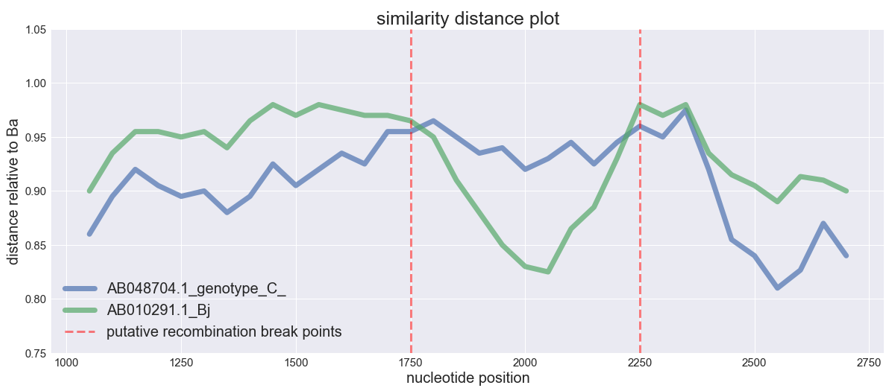
The isolate of Ba genotype is the recombinant between the virus of C genotype and genotype Bj. Let's plot it. We set genotype Ba as the potential recombinant :
```python
sim_obj.simgen(window=200, shift=50, pot_rec=1)
```
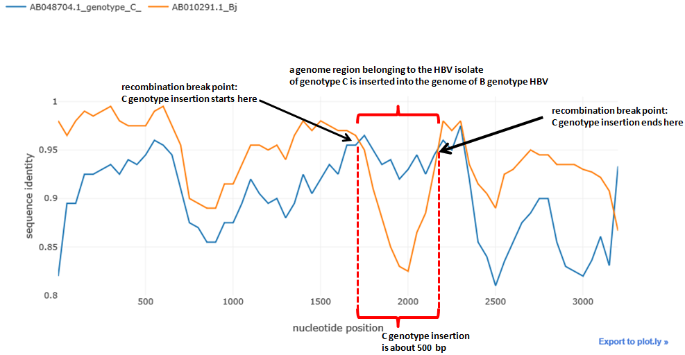
Potential recombinant is not shown in the plot, as the distances are calculated relative to it. The higher is the distance function (i.e. the closer to 1), the closer is the sequence to the recombinant and vice versa.
We can see typical 'crossover' of the distances which is the indicator of the possible recombination event. The distance of one isolate 'drops down' whereas the distance of the other remains the same of even gets closer to the potential recombinant, this abrupt drop shows that recombination could take place.
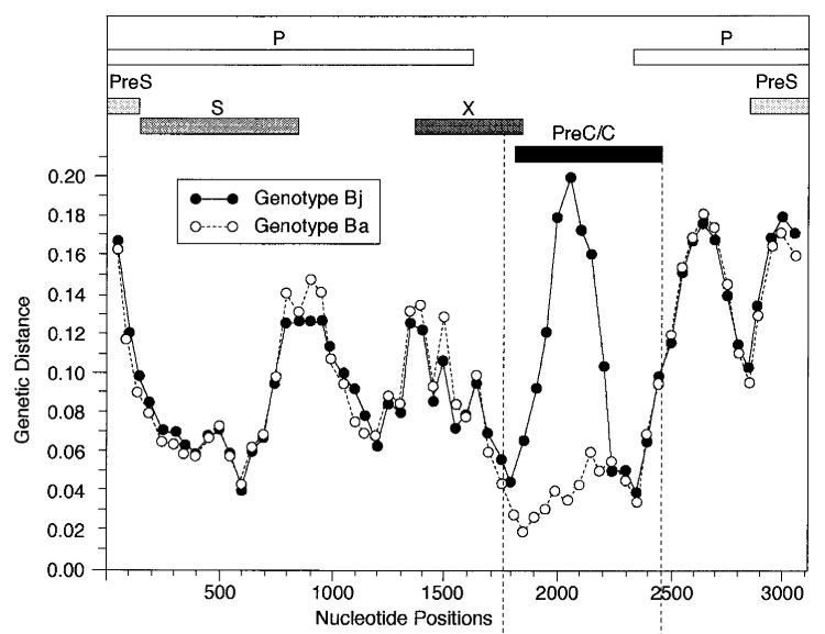
The picture from the article is shown below. It's just turned upside down relative to our plot, and instead of distance drop we see distance rising. Here Bj 'goes away' from the genotype C, whereas Ba keeps the same distance
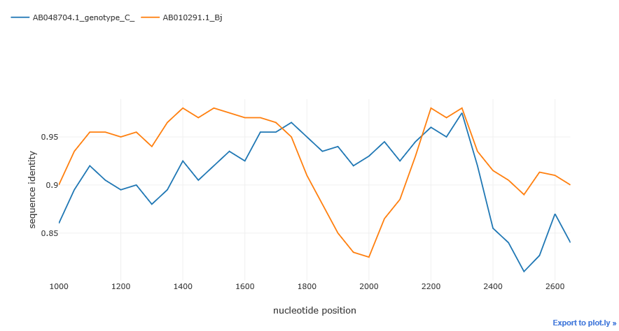
By default `simgen()` method plots the whole alignment. But after initial exploration, we can take a closer look at a particular region by passing the `region` parameter to the simgen method. We can slice the alignment by using this parameter. `region` must be a tuple or a list with two integers: the start and the end position of the alignment slice.
```python
region = (start, end)
```
```python
sim_obj.simgen(window=200, shift=50, pot_rec=1, region=(1000, 2700))
```
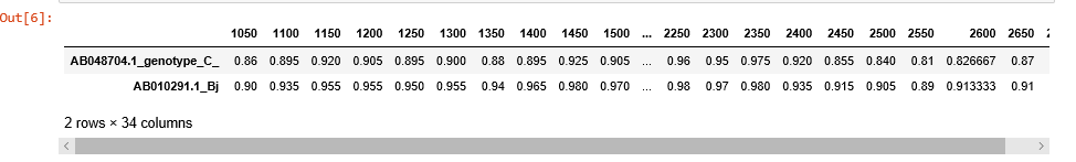
To customize the plot or just to export and store the data, use `get_data()` method. `get_data()` returns pandas DataFrame object with sequences as samples, and distances at given points as features.
```python
sim_obj.get_data()
```
If optional paremeter `df` is set to `False`, `get_data()` returns a tuple containing list of ticks and a dictionary of lists. Each dictionary key is the sequence id, and lists under the keys contain the corresponding distances.
```python
positions, data = sim_obj.get_data(df=False)
```
```
print(positions)
[1050, 1100, 1150, 1200, 1250, 1300, 1350, 1400, 1450, 1500, 1550, 1600, 1650, 1700, 1750, 1800, 1850, 1900, 1950, 2000, 2050, 2100, 2150, 2200, 2250, 2300, 2350, 2400, 2450, 2500, 2550, 2600, 2650, 2700]
print(data)
{'AB048704.1_genotype_C_': [0.88, 0.935, 0.925, 0.955, 0.955, 0.965, 0.95, 0.935, 0.94, 0.92, 0.9299999999999999, 0.945, 0.925, 0.945, 0.96, 0.95, 0.975, 0.9733333333333334, 0.96, 0.96], 'AB010291.1_Bj': [0.98, 0.975, 0.97, 0.97, 0.965, 0.95, 0.91, 0.88, 0.85, 0.83, 0.825, 0.865, 0.885, 0.9299999999999999, 0.98, 0.97, 0.98, 0.9733333333333334, 0.96, 0.96]}
```
Once you've returned the data, you can easily customize the plot by using your favourite plotting library:
```python
dist_data = sim_obj.get_data()
import matplotlib.pyplot as plt
import seaborn as sns
sns.set()
fig_dist1 = plt.figure(figsize=(20, 8))
plt.plot(df.loc["AB048704.1_genotype_C_", : ], lw=7, alpha=0.7, label="AB048704.1_genotype_C_")
plt.plot(df.loc["AB010291.1_Bj", : ], lw=7, alpha=0.7, label="AB010291.1_Bj")
plt.ylim(0.75, 1.05)
plt.title("similarity distance plot", fontsize=25)
plt.ylabel("distance relative to Ba", fontsize=20)
plt.xlabel("nucleotide position", fontsize=20)
plt.xticks(fontsize=15)
plt.yticks(fontsize=15)
plt.axvline(1750, alpha=0.5, color="red", lw=3,
linestyle="dashed", label="putative recombination break points")
plt.axvline(2250, alpha=0.5, color="red", lw=3,
linestyle="dashed" )
plt.legend(prop={"size":20})
plt.show()
```
`simgen()` method has optional parameter `dist` which denoted method used to calculate pairwise distance. By default its value is set to `pdist`, so `simgen()` calculates simple pairwise distance.
Parameters for distance calculation methods:
- `pdist` : pairwise distance (default)
- `jcd` : Jukes-Cantor distance
- `k2p` : Kimura 2-parameter distance
- `td` : Tamura distance
```python
sim_obj.simgen(window=200, shift=50, pot_rec=1, region=(1000, 2700), dist='k2p')
```
to save the distance data in csv format use the method `save_data()`:
```python
sim_obj.save_data(out_name="hbv_distance_data")
```
If there are about 20 or 30 sequences in the input file and their names are long, legend element may hide the plot. So, to be able to analyze many sequences at once, it's better to use short consice sequence names instead of long ones. Like this:
To illustrate how typical breakpoints may look like, here are shown some examples of previously described recombinations in the genomes of different viruses. The fasta alignments used are available at [datasets folder](datasets).
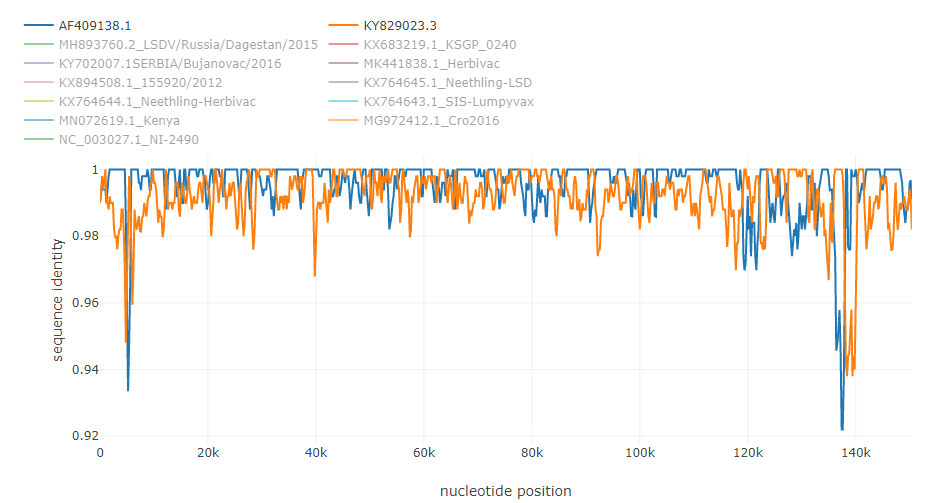
Putative recombinations in the of 145000 bp genome of lumpy skin disease virus [4]:
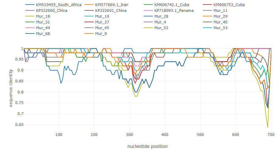
Recombination in HIV genome [5]:
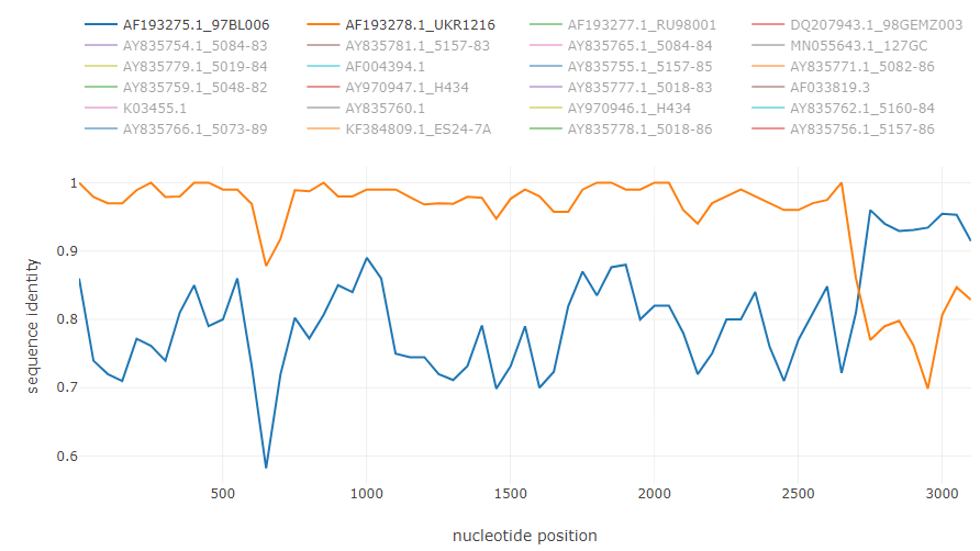
HCV intergenotype recombinant 2k/1b [6]:
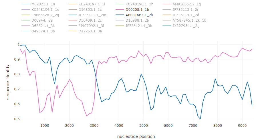
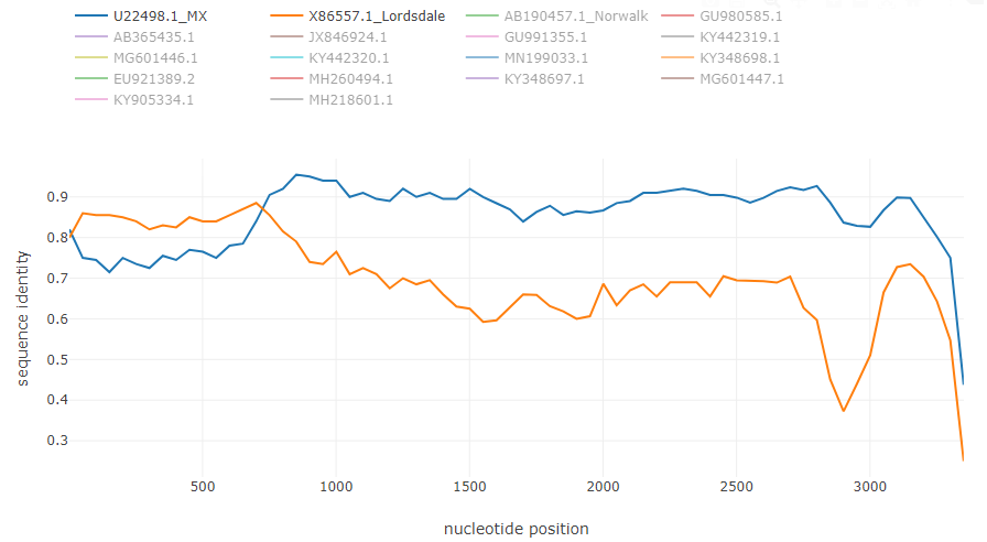
Norovirus recombinant isolate [7]:
## Some notes on usage
- the optimal window size is about 200-250 bp, the optimal window shift is typicall about 50-150 bp
- now distance calculation skips degenerate nucleotides and gaps and they do not influence the distance values
## Automated tests
To verify the installation, go to the `recan/test/` folder and run:
`
$ pytest test.py
`
## Example datasets
To download the datasets use the following link:
https://drive.google.com/drive/folders/1v2lg5yUDFw_fgSiulsA1uFeuzoGz0RjH?usp=sharing
## References
1. Recombination Analysis Tool (RAT): a program for the high-throughput detection of recombination. Bioinformatics, Volume 21, Issue 3,
1 February 2005, Pages 278–281, https://doi.org/10.1093/bioinformatics/bth500
2. https://sray.med.som.jhmi.edu/SCRoftware/simplot/
3. Hepatitis B Virus of Genotype B with or without Recombination with Genotype C over the Precore Region plus the Core Gene. Fuminaka Sugauchi et al. JOURNAL OF VIROLOGY, June 2002, p. 5985–5992. 10.1128/JVI.76.12.5985-5992.2002 https://jvi.asm.org/content/76/12/5985
4. Sprygin A, Babin Y, Pestova Y, Kononova S, Wallace DB, Van Schalkwyk A, et al. (2018) Analysis and insights into recombination signals in lumpy skin disease virus recovered in the field. PLoS ONE 13(12): e0207480. https://doi.org/ 10.1371/journal.pone.0207480
5. Liitsola, K., Holm K., Bobkov, A., Pokrovsky, V., Smolskaya,T., Leinikki,P., Osmanov,S. and Salminen,M. (2000) An AB recombinant and its parental HIV type 1 strains in the area of the former Soviet Union: low requirements for sequence identity in recombination. UNAIDS Virus Isolation Network. AIDS Res. Hum. Retroviruses, 16, 1047–1053.
6. Smith, D. B., Bukh, J., Kuiken, C., Muerhoff, A. S., Rice, C. M., Stapleton, J. T., & Simmonds, P. (2014). Expanded classification of hepatitis C virus into 7 genotypes and 67 subtypes: Updated criteria and genotype assignment web resource. Hepatology, 59(1), 318–327. https://doi.org/10.1002/hep.26744
7. Jiang,X., Espul,C., Zhong,W.M., Cuello,H. and Matson,D.O. (1999) Characterization of a novel human calicivirus that may be a naturally occurring recombinant. Arch. Virol., 144, 2377–2387.
8. Martin, D. P., Murrell, B., Golden, M., Khoosal, A., & Muhire, B. (2015). RDP4: Detection and analysis of recombination patterns in virus genomes. Virus Evolution, 1(1), 1–5. https://doi.org/10.1093/ve/vev003
9. Babin, Y., (2020). Recan: Python tool for analysis of recombination events in viral genomes. Journal of Open Source Software, 5(49), 2014.
https://doi.org/10.21105/joss.02014
## recan citations
1. Zimerman RA, Ferrareze PAG, Cadegiani FA, Wambier CG, Fonseca DdN, de Souza AR, Goren A, Rotta LN, Ren Z and Thompson CE (2022) Comparative Genomics and
Characterization of SARS-CoV-2 P.1 (Gamma) Variant of Concern From Amazonas, Brazil. Front. Med. 9:806611. doi: 10.3389/fmed.2022.806611
2. In book: Proceedings of the 4th International Conference on Big Data Analytics for Cyber-Physical System in Smart City - Volume 2. Chapter: Python Data Analysis Techniques in Administrative Information Integration Management System April 2023 DOI: 10.1007/978-981-99-1157-8_35
|
