---
title: SPARQL Tutorial
short-description: SPARQL Tutorial
...

# SPARQL Tutorial

This tutorial aims to introduce you to RDF and SPARQL from the ground
up. All examples come from the Nepomuk ontology, and even though
the tutorial aims to be generic enough, it mentions things
specific to Tracker, those are clearly spelled out.

If you are reading this tutorial, you might also have Tracker installed
in your system, if that is the case you can for example start a fresh
empty SPARQL service for local testing:

```bash
$ tracker3 endpoint --dbus-service a.b.c --ontology nepomuk
```

The queries can be run in this specific service with:

```bash
$ tracker3 sparql --dbus-service a.b.c --query $SPARQL_QUERY
```

## RDF Triples

RDF data define a graph, composed by vertices and edges. This graph is
directed, because edges point from one vertex to another, and it is
labeled, as those edges have a name. The unit of data in RDF is a
triple of the form:

    subject  predicate  object

Or expressed visually:

![Triple Graph](images/triple-graph-1.png)

Subject and object are 2 graph vertices and the predicate is the edge,
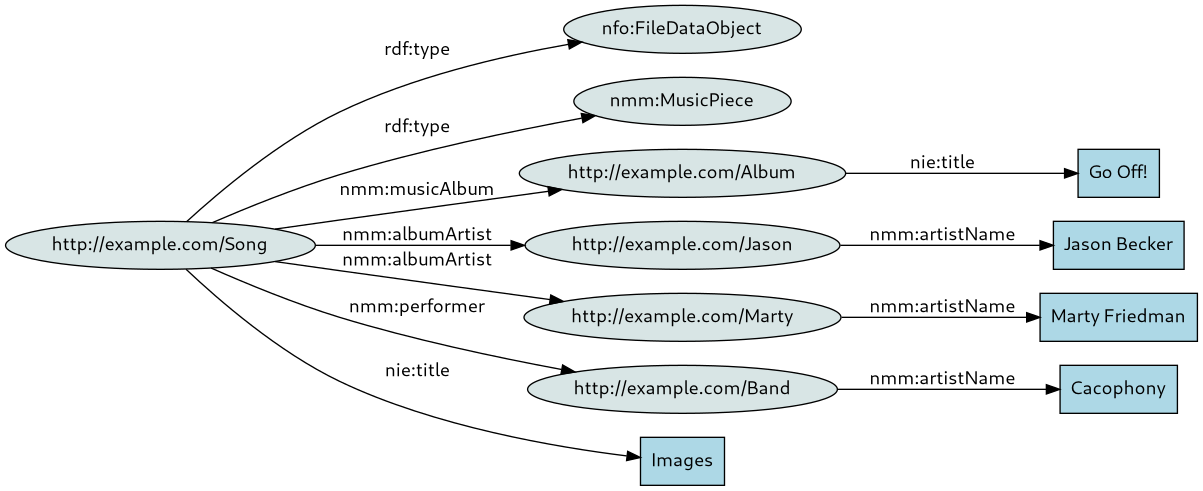
the accumulation of those triples form the full graph. For example,
the following triples:

```turtle
<http://example.com/Song> a nfo:FileDataObject .
<http://example.com/Song> a nmm:MusicPiece .
<http://example.com/Song> nie:title "Images" .
<http://example.com/Song> nmm:musicAlbum <http://example.com/Album> .
<http://example.com/Song> nmm:albumArtist <http://example.com/Jason> .
<http://example.com/Song> nmm:albumArtist <http://example.com/Marty> .
<http://example.com/Song> nmm:performer <http://example.com/Band> .

<http://example.com/Album> a nmm:MusicAlbum .
<http://example.com/Album> nie:title "Go Off!" .

<http://example.com/Jason> a nmm:Artist .
<http://example.com/Jason> nmm:artistName "Jason Becker" .

<http://example.com/Marty> a nmm:Artist .
<http://example.com/Marty> nmm:artistName "Marty Friedman" .

<http://example.com/Band> a nmm:Artist .
<http://example.com/Band> nmm:artistName "Cacophony" .
```

Would visually generate the following graph:

![Triple Graph](images/triple-graph-2.png)

The dot after each triple is not (just) there for legibility, but is
part of the syntax. The RDF triples in full length are quite
repetitive and cumbersome to write, luckily they can be shortened by
providing multiple objects (with `,` separator) or multiple
predicate/object pairs (with `;` separator), the previous RDF could be
shortened into:

```turtle
<http://example.com/Song> a nfo:FileDataObject, nmm:MusicPiece .
<http://example.com/Song> nie:title "Images" .
<http://example.com/Song> nmm:musicAlbum <http://example.com/Album> .
<http://example.com/Song> nmm:albumArtist <http://example.com/Jason> , <http://example.com/Marty> .
<http://example.com/Song> nmm:performer <http://example.com/Band> .

<http://example.com/Album> a nmm:MusicAlbum .
<http://example.com/Album> nie:title "Go Off!" .

<http://example.com/Jason> a nmm:Artist .
<http://example.com/Jason> nmm:artistName "Jason Becker" .

<http://example.com/Marty> a nmm:Artist .
<http://example.com/Marty> nmm:artistName "Marty Friedman" .

<http://example.com/Band> a nmm:Artist .
<http://example.com/Band> nmm:artistName "Cacophony" .
```

And further into:

```turtle
<http://example.com/Song> a nfo:FileDataObject, nmm:MusicPiece ;
    nie:title "Images" ;
    nmm:musicAlbum <http://example.com/Album> ;
    nmm:albumArtist <http://example.com/Jason> , <http://example.com/Marty> ;
    nmm:performer <http://example.com/Band> .

<http://example.com/Album> a nmm:MusicAlbum ;
    nie:title "Go Off!" .

<http://example.com/Jason> a nmm:Artist ;
    nmm:artistName "Jason Becker" .

<http://example.com/Marty> a nmm:Artist ;
    nmm:artistName "Marty Friedman" .

<http://example.com/Band> a nmm:Artist ;
    nmm:artistName "Cacophony" .
```

## SPARQL

SPARQL is the definition of a query language for RDF data. How does a query
language for graphs work? Naturally by providing a graph to be matched, it
is conveniently called the "graph pattern".

SPARQL extends over the RDF concepts and syntax, once familiar with RDF the
basic data insertion syntax should be fairly self-explanatory:

```SPARQL
INSERT DATA {
    <http://example.com/Song> a nfo:FileDataObject, nmm:MusicPiece ;
        nie:title "Images" ;
        nmm:musicAlbum <http://example.com/Album> ;
        nmm:albumArtist <http://example.com/Jason> , <http://example.com/Marty> ;
        nmm:performer <http://example.com/Band> .

    <http://example.com/Album> a nmm:MusicAlbum ;
        nie:title "Go Off!" .

    <http://example.com/Jason> a nmm:Artist ;
        nmm:artistName "Jason Becker" .

    <http://example.com/Marty> a nmm:Artist ;
        nmm:artistName "Marty Friedman" .

    <http://example.com/Band> a nmm:Artist ;
        nmm:artistName "Cacophony" .
}
```

Same with simple data deletion:

```SPARQL
DELETE DATA {
    <http://example.com/Resource> a rdfs:Resource ;
}
```

And simple graph testing:

```SPARQL
# Tell me whether this RDF data exists in the store
ASK {
    <http://example.com/Song> nie:title "Images" ;
        nmm:albumArtist <http://example.com/Jason> ;
        nmm:musicAlbum <http://example.com/Album> .
    <http://example.com/Album> nie:title "Go Off!" .
    <http://example.com/Jason> nmm:artistName "Jason Becker"
}
```

Which would result in `true`, as the triple does exist. The ASK query
syntax results in a single boolean row/column containing whether the
provided graph exists in the store or not.

## Queries and variables

Of course, the deal of a query language is being able to obtain the
stored data, not just testing whether data exists.

The `SELECT` query syntax is used for that, and variables are denoted with
a `?` prefix (or `$`, although that is less widely used), variables act
as "placeholders" where any data will match and be available to the resultset
or within the query as that variable name.

These variables can be set anywhere as the subject, predicate or object of
a triple. For example, the following query could be considered the opposite
to the simple boolean testing the that `ASK` provides:

```SPARQL
# Give me every known triple
SELECT * {
    ?subject ?predicate ?object
}
```

What does this query do? it provides a triple with 3 variables, that
every known triple in the database will match. The `*` is a shortcut
for all queried variables, the query could also be expressed as:

```SPARQL
SELECT ?subject ?predicate ?object {
    ?subject ?predicate ?object
}
```

However, querying for all known data is most often hardly useful, this
got unwieldly soon! Luckily, that is not necessarily the case, the
variables may be used anywhere in the triple definition, with other
triple elements consisting of literals you want to match for, e.g.:

```SPARQL
# Give me the title of the song (Result: "Images")
SELECT ?songName {
    <http://example.com/Song> nie:title ?songName
}
```

```SPARQL
# What is this text to the album? (Result: the nie:title)
SELECT ?predicate {
    <http://example.com/Album> ?predicate "Go Off!"
}
```

```SPARQL
# What is the resource URI of this fine musician? (Result: <http://example.com/Marty>)
SELECT ?subject {
    ?subject nmm:artistName "Marty Friedman"
}
```

```SPARQL
# Give me all resources that are a music piece (Result: <http://example.com/Song>)
SELECT ?song {
    ?song a nmm:MusicPiece
}
```

And also combinations of them, for example:

```SPARQL
# Give me all predicate/object pairs for the given resource
SELECT ?pred ?obj {
    <http://example.com/Song> ?pred ?obj
}
```

```SPARQL
# The Answer to the Ultimate Question of Life, the Universe, and Everything
SELECT ?subj ?pred {
    ?subj ?pred 42
}
```

```SPARQL
# Give me all resources that have a title, and their title.
SELECT ?subj ?obj {
    ?subj nie:title ?obj
}
```

And of course, the graph pattern can hold more complex triple
definitions, that will be matched as a whole across the stored
data. for example:

```SPARQL
# Give me all songs from this fine album
SELECT ?song {
    ?album nie:title "Go Off!" .
    ?song nmm:musicAlbum ?album
}
```

```SPARQL
# Give me all song resources, their title, and their album title
SELECT ?song ?songTitle ?albumTitle {
    ?song a nmm:MusicPiece ;
        nmm:musicAlbum ?album ;
        nie:title ?songTitle .
    ?album nie:title ?albumTitle
}
```

Stop a bit to think on the graph pattern expressed in the last query:
![Graph Pattern](images/triple-graph-3.png)

This pattern on one hand consists of specified data (eg. `?song` must be
a `nmm:MusicPiece`, it must have a `nmm:musicAlbum` and a `nie:title`,
`?album` must have a `nie:title`, which must all apply for a match
to happen.

On the other hand, the graph pattern contains a number of variables,
some only used internally in the graph pattern, as a temporary
variable of sorts (?album, in order to express the relation between
?song and its album title), while other variables are requested in the
result set.

## URIs, URNs and IRIs

In RDF data, everything that can be identified does so by
a URI. URIs uniquely identify an element in the RDF set, have
properties that are defined by URIs themselves, and point to
data that may either be other resources (identified by URI) or
literal values.

Given URIs are central to RDF data and SPARQL queries, there are
a number of ways to write, generalize and shorten them. URIs can
of course be defined in their full form:

```SPARQL
ASK {
    <http://example.com/a> rdf:type rdfs:Resource .
    <http://example.com/sub/b> rdfs:label 'One' .
}
```

Sadly, not everything in the world can be trivially mapped to
a URI, as an aide Tracker offers helpers to generate URIs based
on UUIDv4 identifiers like [](tracker_sparql_get_uuid_urn),
these generated strings are typically called URNs.

The `BASE` keyword allows setting a common prefix for all URIs
in the query:

```SPARQL
BASE <http://example.com/>

ASK {
    <a> rdf:type rdfs:Resource .
    <sub/b> rdfs:label 'One' .
}
```

Or different prefixes can be defined with the `PREFIX` keyword:

```SPARQL
PREFIX ex: <http://example.com/>
PREFIX sub: <http://example.com/sub/>

ASK {
    ex:a rdf:type rdfs:Resource .
    sub:b rdfs:label 'One' .
}
```

Notice how in the first triple, subject/predicate/object now look the
same? That is because they now all are prefixed names, here the `rdf`
and `rdfs` prefixes are simply builtin.

Taking the opposite path (i.e. expanding every term), this query could
be written as:

```SPARQL
ASK {
    <https://example/a> <http://www.w3.org/1999/02/22-rdf-syntax-ns#type> <http://www.w3.org/2000/01/rdf-schema#Resource> .
    <https://example/sub/b> <http://www.w3.org/1999/02/22-rdf-syntax-ns#label> 'One' .
}
```

For the sake of familiarity, these elements have been referred to as
"URIs", but these are actually IRIs, thus the unicode range is available:

```SPARQL
INSERT DATA {
    <http://example.com/💣> a rdfs:Resource
}
```

## Filtering data

With some practice and experimentation, it should be quick to get the hang
of graph patterns, and how do they match the stored RDF data. But it also
quickly comes with the realization that it is completely binary, every piece
of RDF data that matches the graph pattern is returned and everything else
is ignored.

The `FILTER` keyword adds the missing further expressiveness, allowing to
define arbitrary expressions on the variables defined in the graph
pattern. E.g.:

```SPARQL
# Get images larger than 800x600, at 4:3 ratio
SELECT ?image {
    ?image a nfo:Image ;
        nfo:width ?width ;
        nfo:height ?height .
    FILTER (?width > 800 &&
            ?height > 600 &&
            (?width / ?height = 4/3)) .
}
```

Conceptually, every solution given by the graph pattern runs through these
filters, providing finer control over the final set of solutions. These
filters are ultimately interpreted as boolean values, for example the
following query:

```SPARQL
# This returns nothing!
SELECT * {
   ?subject ?predicate ?object .
   FILTER (false)
}
```

Would return no results, as every solution is filtered out.

The SPARQL language also provides a number of
[builtin functions](https://www.w3.org/TR/sparql11-query/#SparqlOps) that
are suitable for use in filters (e.g. for string checks and manipulation),
these complement the relational expressions `= != > >= < <=`.

It is also possible to provide a list of possible values for variables to
be filtered in or out via the operators `IN` and `NOT IN`:

```SPARQL
# Give me every folder, except those named "Music" or "Downloads"
SELECT ?song {
    ?folder a nfo:Folder ;
        nfo:fileName ?name .
    FILTER (?name NOT IN ('Music', 'Downloads'))
}
```

## Aggregate functions

Aggregate functions are those that work over groups of solutions, e.g.:

```SPARQL
# Tell me how many songs do I have
SELECT (COUNT (?song) AS ?count) {
    ?song a nmm:MusicPiece .
}
```

By default, there is a single group for all solutions, a different
grouping can be provided with the `GROUP BY` clause.

```SPARQL
# Get the run time of each of my albums, the sum of their music pieces.
SELECT ?album (SUM (?duration) AS ?runtime) {
    ?song a nmm:MusicPiece ;
        nfo:duration ?duration ;
        nmm:musicAlbum ?album .
}
GROUP BY ?album
```

For numeric operations, SPARQL defines the `COUNT / MIN / MAX / SUM / AVG`
functions. For strings, concatenation is available via the `GROUP_CONCAT`
function. The `SAMPLE` function can be used to pick one of the values at
random.

```SPARQL
# Give me a list of directors, with one of their movies.
SELECT ?director (SAMPLE (?movie) AS ?sample) {
    ?movie a nmm:Movie ;
        nmm:director ?director .
}
GROUP BY ?director
```

Sometimes, it is desirable to apply filters on these aggregate values.
The `HAVING` clause behaves like `FILTER`, except it can be used
to apply filters on these aggregate values:

```SPARQL
# Get music albums, but filter out singles and bonus discs (an arbitrary
# minimum of 4 songs is used for this)
SELECT ?album {
    ?song a nmm:MusicPiece .
        nmm:musicAlbum ?album
}
GROUP BY ?album
HAVING (COUNT (?song) >= 4)
```

## Optional data

As we have seen, the graph pattern provided in `SELECT` queries match as
a whole, stored RDF data either is a match (and becomes a possible solution),
or it does not. Sometimes the available data is not all that regular, so it
is desirable to create a graph pattern that can find solutions where some
variables are left blank.

The `OPTIONAL` clause can be used for this:

```SPARQL
# Get songs, and their known performer(s). But audio files are often mis/unlabeled!
SELECT ?song ?performer {
    ?song a nmm:MusicPiece .
    OPTIONAL {
        ?song nmm:performer ?performer .
    }
}
```

This query will always return all music pieces, but as the song's `nmm:performer`
property is obtained inside the `OPTIONAL` clause, it does not become mandatory
to be part of the set of solutions. Contrast with:

```SPARQL
SELECT ?song ?performer {
    ?song a nmm:MusicPiece ;
        nmm:performer ?performer .
}
```

Which will only return music pieces that have a `nmm:performer`.

It is worth pointing out that the content of `OPTIONAL { }` is itself also a graph
pattern, so it also either matches as a whole or it does not. When fetching multiple
optional properties, it is a common pitfall to do:

```SPARQL
# BAD ❌: Only songs that have both performer *and* composer will match the
# optional graph pattern. Otherwise these 2 variables will be null.
SELECT ?song ?performer ?composer {
    ?song a nmm:MusicPiece .
    OPTIONAL {
        ?song nmm:performer ?performer ;
            nmm:composer ?composer .
    }
}
```

If there are multiple optional pieces of data, these must happen in separate
`OPTIONAL` clauses:

```SPARQL
# GOOD ✅: Songs may have none/either/both of performer/composer.
SELECT ?song ?performer ?composer
    ?song a nmm:MusicPiece .
    OPTIONAL {
        ?song nmm:performer ?performer .
    } .
    OPTIONAL {
        ?song nmm:composer ?composer .
    }
}
```

## Property paths

Up till now, we have been defining triples in the graph pattern as
sets of `subject predicate object`. A single predicate like that
is the simplest property path there is, it relates subject and object
directly via a labeled arrow.

![](images/triple-graph-1.png)

Property paths make it possible to define more complex connections
between subject and object (literally, paths of properties). The `/`
operator may be used for concatenation:

```SPARQL
# Get songs and their performer artist name, jumping across
# the intermediate nmm:Artist resource.
SELECT ?song ?artistName {
    ?song nmm:performer/nmm:artistName ?artistName
}
```

The `|` operator may be used for providing optional paths:

```SPARQL
# Get songs and their performer/composer artist names, jumping across
# the intermediate nmm:Artist resources.
SELECT ?song ?artistName {
    ?song (nmm:performer|nmm:composer)/nmm:artistName ?artistName
}
```

The unary `*` and `+` operators may be used to define recursive paths,
`*` allows a 0-length property path (essentially, subject equals object),
while `+` requires that the property path should happen at least once.

```SPARQL
# Get the XDG music folder, plus all its recursive contents.
SELECT ?file {
    ?file a nfo:FileDataObject ;
        (nfo:belongsToContainer/nie:isStoredAs)* ?root .
    FILTER (?root = 'file:///home/.../Music')
}
```

The unary `?` operator makes portions of the property path optional,
matching paths with either length 0 or 1:

```SPARQL
# Get the XDG music folder, plus all its direct contents.
SELECT ?file {
    ?file a nfo:FileDataObject ;
        (nfo:belongsToContainer/nie:isStoredAs)? ?root .
    FILTER (?root = 'file:///home/.../Music')
}
```

The `^` operator inverts the direction of the relation expressed
by the property path:

```SPARQL
# The arrow goes in the other direction!
SELECT ?song ?artistName {
    ?artistName ^nmm:artistName ?song
}
```

The `!` operator inverts the meaning of the match:

```SPARQL
# Give me everything except the title
SELECT ?song ?value {
    ?song !nie:title ?value .
}
```

These operators may be all nested with `( )`, allowing full
expressiveness when defining the ways subject and object are
interrelated.

## Ontologies

In the RDF world, an "ontology" defines the characteristics of
the data that a RDF database can hold. RDF triples that fit in its
view of the world are accepted, while data that does not is rejected.

```SPARQL
# This is good
INSERT DATA {
    <a> rdf:type rdfs:Resource
};

# This is bad, this property is unknown
INSERT DATA {
    <a> ex:nonExistentProperty 1000
}
```

Tracker defines all its ontologies on top of the RDF Schema, which
provides the basic blocks to define classes (i.e. the types of
the resources being stored) and the properties that each of these
can have.

Basic types and literals have their own builtin classes (e.g.
`xsd:string` for string literals), properties can point to either
one of these builtin classes (e.g. the `rdfs:label` property points
to string literals), or any other class defined in the ontology.
This ability to "define the type" of properties allows to define
the structure of the data:

```SPARQL
# This is consistent, the nmm:musicAlbum property
# must point to a nmm:MusicAlbum resource
INSERT DATA {
    <album> a nmm:MusicAlbum .
    <song1> a nmm:MusicPiece ;
        nmm:musicAlbum <album>
}

# This is inconsistent, agenda contacts are not albums
INSERT DATA {
    <contact> a nco:Contact .
    <song2> a nmm:MusicPiece ;
        nmm:musicAlbum <contact>
}
```

The ontology is defined via RDF itself, and Tracker makes it part
of the data set, there are thus full introspection capabilities
builtin:

```SPARQL
# Query all available classes
SELECT ?class {
    ?class a rdfs:Class
}
```

```SPARQL
# Query all available properties, get
# the class they belong to, and the class
# type they point to.
SELECT ?definedOn ?property ?pointsTo {
    ?property a rdf:Property ;
        rdfs:domain ?definedOn ;
        rdfs:range ?pointsTo .
}
```

It is even possible to use these introspection capabilities while
querying the stored data:

```SPARQL
# Get all string properties of any song.
SELECT ?song ?value {
    ?song a nmm:MusicPiece ;
        ?p ?value .
    ?p rdfs:range xsd:string .
}
```

To learn more about how ontologies are done, read the documentation about
[defining ontologies](ontologies.md). Tracker also provides a stock
[Nepomuk](nepomuk.md) ontology, ready for use.

## Inserting data

Once you know how RDF data is written, and are moderately acquainted with
the ontology used by the database you are targeting, the syntax to insert
data should be quite evident:

```SPARQL
# Add a new music piece
INSERT DATA {
    <song> a nmm:MusicPiece
}
```

Just like with SELECT queries, the RDF data in a `INSERT DATA` clause
may represent complex graphs:

```SPARQL
# Add a new music piece, with more information
INSERT DATA {
    <song> a nmm:MusicPiece ;
        nfo:duration 360 ;
        nfo:codec 'MP3' ;
        nmm:dlnaProfile 'MP3' ;
        nie:title "It's a long way to the top" ;
        nmm:musicAlbum <album> ;
        nmm:artist <artist> .
    <album> a nmm:MusicAlbum ;
        nmm:albumDuration 5000 ;
        nie:title "T.N.T." .
    <artist> nmm:artistName "AC DC" .
}
```

## Updating and deleting data

We have already seen the `INSERT DATA` and `DELETE DATA` syntax
that allows specifying pure RDF data to manipulate the stored
data.

It is additionally possible to perform bulk insertions and deletions
over the already stored data. It is worth introducing first to the
full syntax for updates and deletions:

```SPARQL
DELETE {
   # Triple data
} INSERT {
   # Triple data
} WHERE {
   # Graph pattern
}
```

This query looks for all RDF data that matches the WHERE clause,
and proceeds to deleting and inserting the given triple data for
each of the matches.

The `DELETE` and `INSERT` clauses of this query form are optional,
allowing to simply insert data:

```SPARQL
# My favorite song is... all of them!
INSERT {
    ?song nao:hasTag nao:predefined-tag-favorite .
} WHERE {
    ?song a nmm:MusicPiece .
}
```

Or delete it:

```SPARQL
# Delete all songs
DELETE {
    ?song a rdfs:Resource .
} WHERE {
    ?song a nmm:MusicPiece .
}
```

This last form can be further reduced if the RDF data
to look for is also the data that should be deleted:

```SPARQL
# Delete all songs, again
DELETE WHERE {
    ?song a nmm:MusicPiece, rdfs:Resource .
}
```

Going back to the full query form, there is no relation
required between the data being deleted and the data being
inserted. Its use can range from minor updates:

```SPARQL
# Replace title of a song
DELETE {
    ?song nie:title ?title
} INSERT {
    ?song nie:title 'Two'
} WHERE {
    ?song a nmm:MusicPiece ;
        nie:title ?title .
    FILTER (?title = 'One')
}
```

To outright data substitutions:

```SPARQL
# These are not songs, but personal recordings!
DELETE {
    # Delete anything that makes it look like a music piece
    ?notasong a nmm:MusicPiece .
    ?performer a rdfs:Resource .
    ?composer a rdfs:Resource .
} INSERT {
    # And insert my own data
    ?notasong a nfo:Note ;
        nie:title 'My Notes' .
} WHERE {
    ?notasong a nmm:MusicPiece ;
        nmm:performer ?performer ;
        nmm:composer ?composer .
}
```

## Blank nodes

Blank nodes (or anonymous nodes) are nodes without an specified URI, these
are given a query-local name via the special `_:` prefix:

```SPARQL
# Insert a blank node
INSERT DATA {
    _:anon a nmm:MusicPiece
}
```

Note that running this query multiple times will insert a different blank
node each time. Unlike e.g.:

```SPARQL
INSERT DATA {
    <http://example.com/song1> a nmm:MusicPiece
}
```

Where any second insert would be redundantly attempting to add the same
triple to the store.

By default, Tracker deviates from the SPARQL standard in the handling
of blank nodes, these are considered a generator of URIs. The
[](TRACKER_SPARQL_CONNECTION_FLAGS_ANONYMOUS_BNODES) flag may be used to
make Tracker honor the SPARQL 1.1 standard with those. The standard
defines blank nodes as truly anonymous, you can only use them to determine
that there is something that matches the graph pattern you defined. The
practical difference could be seen with this query:

```SPARQL
SELECT ?u {
    ?u a rdfs:Resource .
    FILTER (isBlank (?u))
}
```

Tracker by default will provide you with URNs that can be fed into other
SPARQL queries as URIs. With [](TRACKER_SPARQL_CONNECTION_FLAGS_ANONYMOUS_BNODES)
enabled, the returned elements will be temporary names that can only be used to
determine the existence of a distinct match. There, blank nodes can match named
nodes, but named nodes do not match with blank nodes.

This nature of blank nodes is however useful to query for elements whose
resource URI is irrelevant, e.g.:

```SPARQL
# Query songs, and their disc's artist name
SELECT ?song ?artistName {
    ?song a nmm:MusicPiece ;
        nmm:musicAlbum _:album .
    _:album a nmm:MusicAlbum ;
        nmm:albumArtist _:artist ;
    _:artist a nmm:Artist ;
        nmm:artistName ?artistName .
}
```

In this query there is no interest in getting the intermediate album
and artist resources, so blank nodes can be used for them.

Blank nodes have an in-place `[ ]` syntax, which declares a distinct
empty blank node, it can also contain predicate/object pairs to further
define the structure of the blank node. E.g. the previous query could
be rewritten like:

```SPARQL
SELECT ?song ?artistName {
    ?song a nmm:MusicPiece ;
        nmm:musicAlbum [
            a nmm:MusicAlbum ;
            nmm:albumArtist [
                a nmm:Artist ;
                nmm:artistName ?artistName
            ]
        ]
}
```

## Named graphs

If SPARQL had a motto, it would be "Everything is a graph". Until
this point of the tutorial we have been talking about a singular "graph",
the triple store holds "a graph", graph patterns match against "the graph",
et cetera.

This is not entirely accurate, or rather, it is an useful simplification.
SPARQL is actually able to work over sets of graphs, or their
union/intersection.

As with everything that has a name in RDF, URIs are also used to reference
named graphs. The `GRAPH` clause is used to specify the named graph, in
either inserts/deletes:

```SPARQL
INSERT DATA {
    GRAPH <http://example.com/MyGraph> {
        <http://example.com/MySong> a nmm:MusicPiece ;
            nie:title "My song" .
    }
}
```

Or in queries:

```SPARQL
SELECT ?song {
    GRAPH <http://example.com/MyGraph> {
        ?song a nmm:MusicPiece .
    }
}
```

So what have been doing all these queries up to this point in the tutorial?
Without any specified graph, all insertions and deletes happen on an anonymous
graph, while all queries happen on a "default" graph that Tracker defines as
the union of all graphs.

These named graphs can exist independently of each other, and they can also
overlap (e.g. specific RDF triples may exist in more than one graph). This
makes it possible to match for specific pieces of data in specific graphs:

```SPARQL
# Get info from different graphs, ?file is known in both of them, but none
# has the full information.
SELECT ?fileName ?title {
    GRAPH tracker:FileSystem {
        ?file a nfo:FileDataObject ;
            nfo:fileName ?fileName .
    }
    GRAPH tracker:Pictures {
        ?photo a nmm:Photo ;
            nie:isStoredAs ?file ;
            nie:title ?title .
    }
}
```

Tracker heavily relies on these named graph characteristics for its
sandboxing support, where the availability of graphs may be restricted.

It is also possible to use the `GRAPH` clause with a variable, making it
possible to query for the graph(s) where the graph pattern solutions are
found:

```SPARQL
# Query all known graphs, everything matches an empty graph pattern!
SELECT ?graph { GRAPH ?graph { } }
```

## Services

RDF triple stores are sometimes available as "endpoints", distinct
services available externally via HTTP or other remote protocols, able
to run SPARQL queries.

The SPARQL language itself defines the interoperation with other such
endpoints within SPARQL queries. Since everything is RDF data, and
everything is identified with a URI, this "foreign" RDF data might be
conceptually dealt with as just another graph:

```SPARQL
# Get data from the wikidata SPARQL service for my local albums, using
# an intermediate external reference.
SELECT ?album ?wikiPredicate ?wikiObject {
    ?album a nfo:MusicAlbum ;
        tracker:externalReference ?externalReference .
    ?externalReference tracker:referenceSource 'wikidata' .

    SERVICE <http://query.wikidata.org/sparql> {
        ?externalReference ?wikiPredicate ?wikiObject
    }
}
```

Tracker provides means to make RDF triple stores publicly available as SPARQL
endpoints both via HTTP(S) and D-Bus protocols. By default, triple stores
are not exported as endpoints, and are considered private to a process.

## Importing and exporting data

Bulk insertions of RDF data are available with the `LOAD` clause:

```SPARQL
# Load a file containing RDF data into a named graph
LOAD <file:///path/to/data.rdf> INTO GRAPH <http://example.com/MyGraph>
```

Bulk extraction of data can be obtained with the `DESCRIBE` query clause,
the following query would return all subject/predicate/object triples inserted
by the previous `LOAD` clause:

```SPARQL
# Describe all objects in the named graph
DESCRIBE ?resource {
    GRAPH <http://example.com/MyGraph> {
        ?resource a rdfs:Resource .
    }
}
```

The `DESCRIBE` syntax can also be used to get all triple information describing
specific resources:

```SPARQL
# Get all information around the XDG music folder's URI
DESCRIBE <file:///.../Music>
```

The data returned by `DESCRIBE` is RDF triple data, so it can be serialized as
such.

There may also be situations where it is convenient to transform data to other
RDF formats (e.g. a different ontology) from the get go, the `CONSTRUCT` syntax
exists for this purpose:

```SPARQL
# Convert portions of the Nepomuk ontology into another fictional one.
PREFIX ex: <http://example.com>
CONSTRUCT {
    ?file ex:newTitleProperty ?title ;
        ex:newFileNameProperty ?fileName .
} WHERE {
    ?song a nmm:MusicPiece ;
        nie:isStoredAs ?file ;
        nie:title ?title .
}
```

The data returned by this syntax is also triple data, but ready for consumption
in the other end.

## Conclusion

SPARQL is a rather deep language that takes its purpose (making it possible
to query information in RDF data graphs) very thoroughly, it also has some
unusual features that make it able to scale from small private databases
to large distributed ones.

This is not all that there is, and perhaps the "everything is a graph" mindset
takes a while to think intuitively about to anyone with a background in
relational databases. The purpose that this tutorial hopefully achieved is
that SPARQL queries will now look familiar, and became approachable to reason
about.